Interpret Sum Optimization Output
When you review sum optimization results, the default layout displays all the optimization results and results for specific solutions.
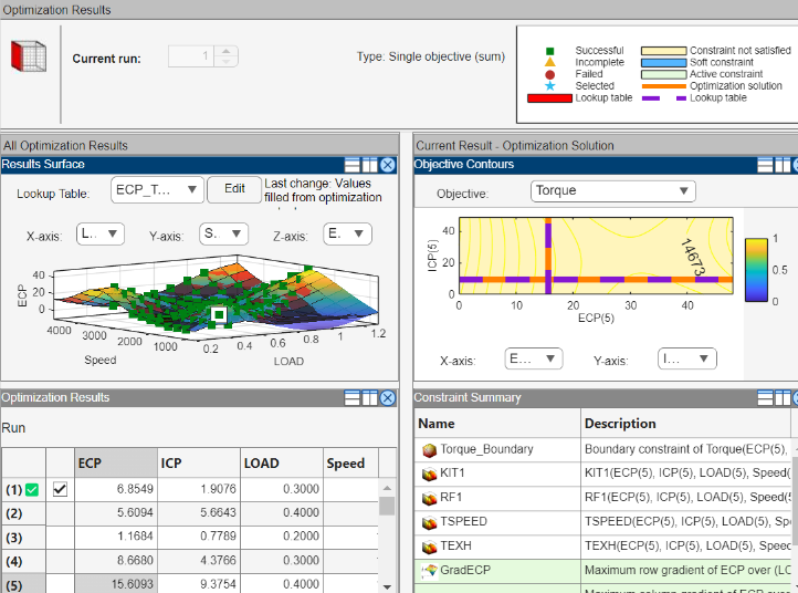
The left side of the layout shows the Results Surface and Optimization Results views for all the results. If you select a run, the:
Objective Contours and Constraint Summary views provides the optimization results.
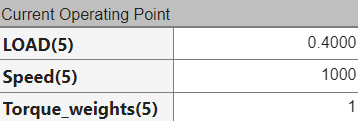
Current Operating Point pane shows the operating point.
In any view, you can change the view by right-clicking and selecting Current View to see the view options.
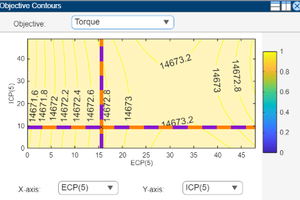
Objective Contour Plot
The objective contour plot for sum objective problems shows the contours of the
objective. You can display plots against any pair of control parameters at each point in
the set of operating points within each run. In this figure, a contour plot shows the
results for run index 5.
Constraint Summary
The Constraint Summary for sum optimizations shows a summary of all the constraint outputs for each constraint at the optimized control parameter settings for the selected run.
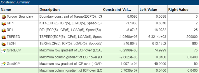
The rows of the table show a summary at each operating point. In this case, each of
the rows corresponds to an evaluation of the constraint at each operating point within
the run. For example, the GradECP constraint rows provide an
evaluation of the maximum row and column gradients of ECP over load.
Optimization Results Table
Features of the Optimization Results table are labeled in this figure.
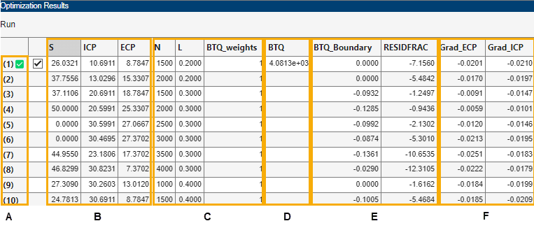
Key to Optimization Results Table
A: The quantity index.
For fixed and free variables, corresponds to the index of the operating point within the run.
For objectives, corresponds to the index of the output for the specific labeled objective.
For constraints, corresponds to the index of the output for the specific labeled constraint.
B: Optimal Optimization Variable Settings — The optimal settings in this case of S, ICP, and ECP at each operating point in the run. For example, the optimal settings of S, ICP and ECP at the third operating point in this run 1 are
S= 37.1106°,ICP= 20.6911°,ECP= 18.7847°.C: Fixed Variable Settings — Settings define the operating points for the run and other fixed variables (such as weights) required for objectives and constraints. These values were set up before the optimization was run.
D: Optimal objective outputs — Optimal values of any objective outputs, that is, the optimized value of the weighted sum of
BTQ(4081.3 Nm) over the 43 operating points shown in this case.E,F: Constraint outputs at optimized control parameter settings — The value of constraint outputs are displayed here. For the example problem, the model constraint outputs are displayed in the section labeled E. The number of constraint outputs matches the number of operating points. The table gradient constraint outputs are displayed in the section labeled F. The number of values returned by the table gradient constraint depends on the internal settings of that constraint.
Operating Point Indices
As in the Input Variable Values pane in the Optimization view, in the output view, the number in the bracket indicates the index of the operating point within a run.
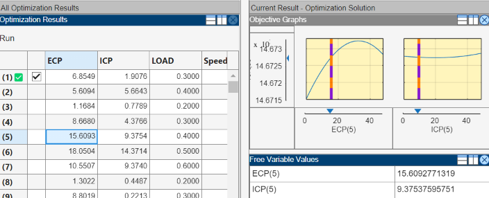
In the Optimization Results table, the index of the operating point
within the run is shown in brackets. In the Free Variable Values table and graphical
displays, InputVariableName(i) provides the input variable at
the i-th operating point within a run. For example, ECP(5) is the
exhaust cam phase at the 5th operating point, and ICP(5) is the
intake cam phase at the first operating point.
You can also use the Current Operating Point table located on the right side of the layout to view the index of the selected operating point.
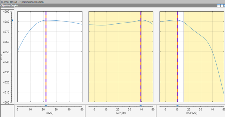
Objective Graphs
The objective graphs for sum objective problems show the objective cross section plots as in
the point case. However, plots are now displayed against each control parameter at each
point in the set of operating points within each run. In this figure, the weighted sum
of BTQ is plotted against the S, ICP, and ECP for operating point
20 in run 1.
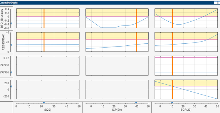
Constraint Graphs
The constraint graphs for sum objective problems show the cross section plots of the left side of the constraints as in the point case. However, in the sum case there are several more inputs and outputs that can be plotted. Specifically, each constraint can return several outputs. You can display the outputs against each control parameter at each point in the set of operating points within each run.