Control of Quadrotor Using Nonlinear Model Predictive Control
This example shows how to design a controller that tracks a trajectory for a quadrotor, using nonlinear model predictive control (MPC).
Quadrotor Model
The quadrotor has four rotors which are directed upwards. From the center of mass of the quadrotor, rotors are placed in a square formation with equal distance. The mathematical model for the quadrotor dynamics is expressed using Euler–Lagrange equations [1].
The twelve states for the quadrotor are:
,
where
denote the positions in an inertial reference frame.
Angle positions are in the roll, pitch, and yaw, respectively.
The remaining states are the velocities of the positions and angles.
The control inputs (also called Manipulated Variables, and indicated as MVs) for the quadrotor are the squared angular velocities of the four rotors:
.
These control inputs create force, torque, and thrust in the direction of the body -axis. In this example, every state is measurable, and the control inputs are constrained to be within [0,10] .
The nonlinear model predictive controller uses a prediction model which comprise a state function (expressing the state derivatives as a function of current state and input) and, when available, a state Jacobians function (expressing the derivatives of the state function with respect to state and input, respectively). Both functions are built and derived using Symbolic Math Toolbox™ software. For more details, see Derive Quadrotor Dynamics for Nonlinear Model Predictive Control (Symbolic Math Toolbox).
Call the script getQuadrotorDynamicsAndJacobian to generate and write to a file both the state and its Jacobians functions.
getQuadrotorDynamicsAndJacobian;
The getQuadrotorDynamicsAndJacobian script generates the following files:
QuadrotorStateFcn.m— State functionQuadrotorStateJacobianFcn.m— State Jacobian function
For details on either function, open the corresponding file.
Design Nonlinear Model Predictive Controller
Create a nonlinear MPC object with 12 states, 12 outputs, and 4 inputs. By default, all the inputs are manipulated variables (MVs).
nx = 12;
ny = 12;
nu = 4;
nlmpcobj = nlmpc(nx, ny, nu);
Zero weights are applied to one or more OVs because there are fewer MVs than OVs.
Specify the prediction model state function using the function name. You can also specify functions using a function handle.
nlmpcobj.Model.StateFcn = "QuadrotorStateFcn";It is best practice to provide an analytical Jacobian for the prediction model. Doing so significantly improves simulation efficiency. Specify the function that returns the Jacobians of the state function using a function handle.
nlmpcobj.Jacobian.StateFcn = @QuadrotorStateJacobianFcn;
Fix the random generator seed for reproducibility.
rng(0)
To check that your prediction model functions for nlobj are valid, use validateFcns for a random point in the state-input space.
validateFcns(nlmpcobj,rand(nx,1),rand(nu,1));
Model.StateFcn is OK.
Jacobian.StateFcn is OK.
No output function specified. Assuming "y = x" in the prediction model.
Analysis of user-provided model, cost, and constraint functions complete.
Specify a sample time of 0.1 seconds, a prediction horizon of 18 steps, and control horizon of 2 steps.
Ts = 0.1;
p = 18;
m = 2;
nlmpcobj.Ts = Ts;
nlmpcobj.PredictionHorizon = p;
nlmpcobj.ControlHorizon = m;
Limit all four control inputs to be in the range [0,10]. Also limit control input change rates to the range [-2,2] to prevent abrupt and rough movements.
nlmpcobj.MV = struct( ...
    Min={0;0;0;0}, ...
    Max={10;10;10;10}, ...
    RateMin={-2;-2;-2;-2}, ...
    RateMax={2;2;2;2} ...
    );
The default cost function in nonlinear MPC is a standard quadratic cost function suitable for reference tracking and disturbance rejection. In this example, the first 6 states are required to follow a given reference trajectory. Because the number of MVs (four) is smaller than the number of reference output trajectories (six), there are not enough degrees of freedom to independently track trajectories for all outputs.
nlmpcobj.Weights.OutputVariables = [1 1 1 1 1 1 0 0 0 0 0 0];
In this example, MVs also have nominal targets (to be set later for the simulation). These targets, which are averages that are set to keep the quadrotor floating when no tracking is required, can lead to conflict between the MV and OV reference tracking goals. To prioritize OV targets, set the average MV tracking priority lower than the average OV tracking priority.
nlmpcobj.Weights.ManipulatedVariables = [0.1 0.1 0.1 0.1];
Also, penalize overly aggressive control actions by specifying tuning weights for the MV rates of change.
nlmpcobj.Weights.ManipulatedVariablesRate = [0.1 0.1 0.1 0.1];
Closed-Loop Simulation
Simulate the system for 20 seconds with a target trajectory to follow.
% Specify the initial conditions
x = [7;-10;0;0;0;0;0;0;0;0;0;0];

% Nominal control target (average to keep quadrotor floating)
nlopts = nlmpcmoveopt;
nlopts.MVTarget = [4.9 4.9 4.9 4.9];
mv = nlopts.MVTarget;
Simulate the closed-loop system using the nlmpcmove function, specifying simulation options using an nlmpcmove object.
% Simulation duration in seconds
Duration = 20;

% Display waitbar to show simulation progress
hbar = waitbar(0,"Simulation Progress");

% MV last value is part of the controller state
lastMV = mv;

% Store states for plotting purposes
xHistory = x';
uHistory = lastMV;

% Simulation loop
for k = 1:(Duration/Ts)

    % Set references for previewing
    t = linspace(k*Ts, (k+p-1)*Ts,p);
    yref = QuadrotorReferenceTrajectory(t);

    % Compute control move with reference previewing
    xk = xHistory(k,:);
    [uk,nlopts,info] = nlmpcmove(nlmpcobj,xk,lastMV,yref',[],nlopts);

    % Store control move
    uHistory(k+1,:) = uk';
    lastMV = uk;

    % Simulate quadrotor for the next control interval (MVs = uk)
    ODEFUN = @(t,xk) QuadrotorStateFcn(xk,uk);
    [TOUT,XOUT] = ode45(ODEFUN,[0 Ts], xHistory(k,:)');

    % Update quadrotor state
    xHistory(k+1,:) = XOUT(end,:);

    % Update waitbar
    waitbar(k*Ts/Duration,hbar);
end

% Close waitbar
close(hbar)
Visualization and Results
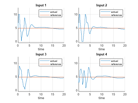
Plot the results, and compare the planned and actual closed-loop trajectories.
plotQuadrotorTrajectory;
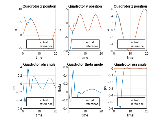
Because the number of MVs is smaller than the number of reference output trajectories, there are not enough degrees of freedom to track the desired trajectories for all OVs independently.
As shown in the figure for states and control inputs,
The states match the reference trajectory very closely within 7 seconds.
The states are driven to the neighborhood of zeros within 9 seconds.
The control inputs are driven to the target value of 4.9 around 10 seconds.
You can animate the trajectory of the quadrotor. The quadrotor moves close to the "target" quadrotor which travels along the reference trajectory within 7 seconds. After that, the quadrotor follows closely the reference trajectory. The animation terminates at 20 seconds.
animateQuadrotorTrajectory;

Conclusion
This example shows how to design a nonlinear model predictive controller for trajectory tracking of a quadrotor. The dynamics and Jacobians of the quadrotor are derived using Symbolic Math Toolbox software. The quadrotor tracks the reference trajectory closely.
References
[1] Raffo, Guilherme V., Manuel G. Ortega, and Francisco R. Rubio. "An integral predictive/nonlinear control structure for a quadrotor helicopter". Automatica 46, no. 1 (January 2010): 29–39. https://doi.org/10.1016/j.automatica.2009.10.018.
[2] Tzorakoleftherakis, Emmanouil, and Todd D. Murphey. "Iterative sequential action control for stable, model-based control of nonlinear systems." IEEE Transactions on Automatic Control 64, no. 8 (August 2019): 3170–83. https://doi.org/10.1109/TAC.2018.2885477.
[3] Luukkonen, Teppo. "Modelling and control of quadcopter". Independent research project in applied mathematics, Aalto University, 2011.
See Also
Functions
Objects
Topics
- Derive Quadrotor Dynamics for Nonlinear Model Predictive Control (Symbolic Math Toolbox)
- Nonlinear MPC