Explicit MPC Control of an Inverted Pendulum on a Cart
This example uses an explicit model predictive controller (explicit MPC) to control an inverted pendulum on a cart.
Pendulum/Cart Assembly
The plant for this example is the following cart/pendulum assembly, where x is the cart position and theta is the pendulum angle.
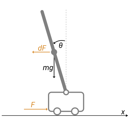
This system is controlled by exerting a variable force F on the cart. The controller needs to keep the pendulum upright while moving the cart to a new position or when the pendulum is nudged forward by an impulse disturbance dF applied at the upper end of the inverted pendulum.
System Equations
The system is described by the following equations, where l is the distance to the pendulum center of mass, m and M are the masses of the pendulum and the cart, respectively, and Kd is a viscous friction damping term.
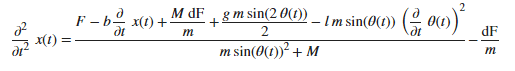
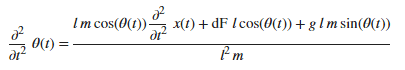
For a thorough explanation of how the equations are derived, see Derive Equations of Motion and Simulate Cart-Pole System (Symbolic Math Toolbox).
These equations are represented in Simulink® with commonly used blocks.
mdlPlant = 'mpc_pendcartPlant';
load_system(mdlPlant)
open_system([mdlPlant '/Pendulum and Cart System'],'force')

This plant is modeled in Simulink with commonly used blocks.
mdlPlant = 'mpc_pendcartPlant';
load_system(mdlPlant)
open_system([mdlPlant '/Pendulum and Cart System'],'force')
Control Objectives
Assume the following initial conditions for the cart/pendulum assembly:
The cart is stationary at x =
0.
The inverted pendulum is stationary at the upright position theta =
0.
The control objectives are:
Cart can be moved to a new position between
-10and10with a step setpoint change.
When tracking such a setpoint change, the rise time should be less than 4 seconds (for performance) and the overshoot should be less than
5percent (for robustness).
When an impulse disturbance of magnitude of
2is applied to the pendulum, the cart should return to its original position with a maximum displacement of1. The pendulum should also return to the upright position with a peak angle displacement of15degrees (0.26radian).
The upright position is an unstable equilibrium for the inverted pendulum, which makes the control task more challenging.
Control Structure
For this example, use a single MPC controller with:
One manipulated variable: variable force F.
Two measured outputs: Cart position x and pendulum angle theta.
One unmeasured disturbance: Impulse disturbance dF.
mdlMPC = 'mpc_pendcartExplicitMPC';
open_system(mdlMPC)

Although cart velocity x_dot and pendulum angular velocity theta_dot are available from the plant model, to make the design case more realistic, they are excluded as MPC measurements.
While the cart position setpoint varies (step input), the pendulum angle setpoint is constant (0 = upright position).
Linear Plant Model
Since the MPC controller requires a linear time-invariant (LTI) plant model for prediction, linearize the Simulink plant model at the initial operating point.
Specify linearization input and output points.
io(1) = linio([mdlPlant '/dF'],1,'openinput');
io(2) = linio([mdlPlant '/F'],1,'openinput');
io(3) = linio([mdlPlant '/Pendulum and Cart System'],1,'openoutput');
io(4) = linio([mdlPlant '/Pendulum and Cart System'],3,'openoutput');
Create operating point specifications for the plant initial conditions.
opspec = operspec(mdlPlant);
The first state is cart position x, which has a known initial state of 0.
opspec.States(1).Known = true;
opspec.States(1).x = 0;
The third state is pendulum angle theta, which has a known initial state of 0.
opspec.States(3).Known = true;
opspec.States(3).x = 0;
Compute operating point using these specifications.
options = findopOptions('DisplayReport',false);
op = findop(mdlPlant,opspec,options);
Obtain the linear plant model at the specified operating point.
plant = linearize(mdlPlant,op,io);
plant.InputName = {'dF';'F'};
plant.OutputName = {'x';'theta'};
Examine the poles of the linearized plant.
pole(plant)
ans =

         0
  -11.9115
   -3.2138
    5.1253
The plant has an integrator and an unstable pole.
bdclose(mdlPlant)
Traditional (Implicit) MPC Design
The plant has two inputs, dF and F, and two outputs, x and theta. In this example, dF is specified as an unmeasured disturbance used by the MPC controller for better disturbance rejection. Set the plant signal types.
plant = setmpcsignals(plant,'ud',1,'mv',2);
To control an unstable plant, the controller sample time cannot be too large (poor disturbance rejection) or too small (excessive computation load). Similarly, the prediction horizon cannot be too long (the plant unstable mode would dominate) or too short (constraint violations would be unforeseen). Use the following parameters for this example:
Ts = 0.01;
PredictionHorizon = 50;
ControlHorizon = 5;
mpcobj = mpc(plant,Ts,PredictionHorizon,ControlHorizon);
-->"Weights.ManipulatedVariables" is empty. Assuming default 0.00000.
-->"Weights.ManipulatedVariablesRate" is empty. Assuming default 0.10000.
-->"Weights.OutputVariables" is empty. Assuming default 1.00000.
   for output(s) y1 and zero weight for output(s) y2
There is a limitation on how much force we can apply to the cart, which is specified as hard constraints on manipulated variable F.
mpcobj.MV.Min = -200;
mpcobj.MV.Max = 200;
It is good practice to scale plant inputs and outputs before designing weights. In this case, since the range of the manipulated variable is greater than the range of the plant outputs by two orders of magnitude, scale the MV input by 100.
mpcobj.MV.ScaleFactor = 100;
To improve controller robustness, increase the weight on the MV rate of change from 0.1 to 1.
mpcobj.Weights.MVRate = 1;
To achieve balanced performance, adjust the weights on the plant outputs. The first weight is associated with cart position x and the second weight is associated with angle theta.
mpcobj.Weights.OV = [1.2 1];
To achieve more aggressive disturbance rejection, increase the state estimator gain by multiplying the default disturbance model gains by a factor of 10.
Update the input disturbance model.
disturbance_model = getindist(mpcobj);
setindist(mpcobj,'model',disturbance_model*10);
-->Converting model to discrete time.
-->The "Model.Disturbance" property is empty:
   Assuming unmeasured input disturbance #1 is integrated white noise.
   Assuming no disturbance added to measured output #1.
-->Assuming output disturbance added to measured output #2 is integrated white noise.
-->"Model.Noise" is empty. Assuming white noise on each measured output.
Update the output disturbance model.
disturbance_model = getoutdist(mpcobj);
setoutdist(mpcobj,'model',disturbance_model*10);
-->Converting model to discrete time.
   Assuming no disturbance added to measured output #1.
-->Assuming output disturbance added to measured output #2 is integrated white noise.
-->"Model.Noise" is empty. Assuming white noise on each measured output.
Explicit MPC Generation
A simple implicit MPC controller, without the need for constraint or weight changes at run-time, can be converted into an explicit MPC controller with the same control performance. The key benefit of using Explicit MPC is that it avoids real-time optimization, and as a result, is suitable for industrial applications that demand fast sample time. The tradeoff is that explicit MPC has a high memory footprint because optimal solutions for all feasible regions are pre-computed offline and stored for run-time access.
To generate an explicit MPC controller from an implicit MPC controller, define the ranges for parameters such as plant states, references, and manipulated variables. These ranges should cover the operating space for which the plant and controller are designed, to your best knowledge.
range = generateExplicitRange(mpcobj);
range.State.Min(:) = -20;   % largest range comes from cart position x
range.State.Max(:) = 20;
range.Reference.Min = -20;  % largest range comes from cart position x
range.Reference.Max = 20;
range.ManipulatedVariable.Min = -200;
range.ManipulatedVariable.Max = 200;
-->Converting model to discrete time.
-->"Model.Noise" is empty. Assuming white noise on each measured output.
Generate an explicit MPC controller for the defined ranges.
mpcobjExplicit = generateExplicitMPC(mpcobj,range);
Regions found / unexplored: 92/ 0
To use the explicit MPC controller in Simulink, specify it in the Explicit MPC Controller block dialog in your Simulink model.
Closed-Loop Simulation
Validate the MPC design with a closed-loop simulation in Simulink.
open_system([mdlMPC '/Scope'])
sim(mdlMPC)


In the nonlinear simulation, all the control objectives are successfully achieved.
Comparing with the results from MPC Control of an Inverted Pendulum on a Cart, the implicit and explicit MPC controllers deliver identical performance as expected.
Discussion
It is important to point out that the designed MPC controller has its limitations. For example, if you increase the step setpoint change to 15, the pendulum fails to recover its upright position during the transition.
To reach the longer distance within the same rise time, the controller applies more force to the cart at the beginning. As a result, the pendulum is displaced from its upright position by a larger angle such as 60 degrees. At such angles, the plant dynamics differ significantly from the LTI predictive model obtained at theta = 0. As a result, errors in the prediction of plant behavior exceed what the built-in MPC robustness can handle, and the controller fails to perform properly.
A simple workaround to avoid the pendulum falling is to restrict pendulum displacement by adding soft output constraints to theta and reducing the ECR weight on constraint softening.
mpcobj.OV(2).Min = -pi/2;
mpcobj.OV(2).Max = pi/2;
mpcobj.Weights.ECR = 100;
However, with these new controller settings, it is no longer possible to reach the longer distance within the required rise time. In other words, controller performance is sacrificed to avoid violation of soft output constraints.
To reach longer distances within the same rise time, the controller needs more accurate models at different angle to improve prediction. Another example Gain-Scheduled MPC Control of Inverted Pendulum on Cart shows how to use gain scheduling MPC to achieve the longer distances.
Close the Simulink model.
bdclose(mdlMPC)
See Also
Functions
generateExplicitMPC|generateExplicitRange|generateExplicitOptions|simplify|generatePlotParameters|plotSection|mpcmoveExplicit|sim
Objects
mpc|explicitMPC|mpcstate
Blocks
Topics
- MPC Control of Aircraft with Unstable Poles
- Explicit MPC Control of a Single-Input-Single-Output Plant
- Explicit MPC Control of DC Servomotor with Constraint on Unmeasured Output
- MPC Control of an Inverted Pendulum on a Cart
- Derive Equations of Motion and Simulate Cart-Pole System (Symbolic Math Toolbox)
- Explicit MPC
- Design Workflow for Explicit MPC
- What Is Model Predictive Control?