Switching Controllers Based on Optimal Costs
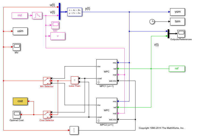
This example shows how to use the "optimal cost" outport of the MPC Controller block to switch between multiple model predictive controllers whose outputs are restricted to discrete values.
Define Plant Model
The linear plant model is as follows:
% Plant with 2 inputs and 1 output
plant = ss(tf({1,1},{[1 1.2 1],[1 1]}),'min');

% Get state-space realization matrices, to be used in Simulink(R)
[A,B,C,D] = ssdata(plant);

% Initial plant state
x0 = [0;0;0];
Design MPC Controller
Specify input and output signal types.
 % The first input is the manipulated variable, the second is measured disturbance
plant = setmpcsignals(plant,'MV',1,'MD',2);
Design two MPC controllers with two equality constraints on the manipulated variable, of u=-1 for the first one and u=1 for the second one. Only u at the current time is quantized. The subsequent calculated control actions might be any value between -1 and 1. The controller uses a receding horizon approach so these values don't actually go to the plants.
Ts = 0.2;                                             % Sampling time
p = 20;                                               % Prediction horizon
m = 10;                                               % Control horizon
mpc1 = mpc(plant,Ts,p,m);                             % First MPC object
mpc2 = mpc(plant,Ts,p,m);                             % Second MPC object

% Specify weights
mpc1.Weights = struct('MV',0,'MVRate',.3,'Output',1);   % Weights
mpc2.Weights = struct('MV',0,'MVRate',.3,'Output',1);   % Weights

% Specify constraints

% Constraints on the manipulated variable for the first controller: u = -1
mpc1.MV = struct('Min',[-1;-1],'Max',[-1;1]);

% Constraints on the manipulated variable for the second controller: u = 1
mpc2.MV = struct('Min',[1;-1],'Max',[1;1]);
-->"Weights.ManipulatedVariables" is empty. Assuming default 0.00000.
-->"Weights.ManipulatedVariablesRate" is empty. Assuming default 0.10000.
-->"Weights.OutputVariables" is empty. Assuming default 1.00000.
-->"Weights.ManipulatedVariables" is empty. Assuming default 0.00000.
-->"Weights.ManipulatedVariablesRate" is empty. Assuming default 0.10000.
-->"Weights.OutputVariables" is empty. Assuming default 1.00000.
Simulate in Simulink
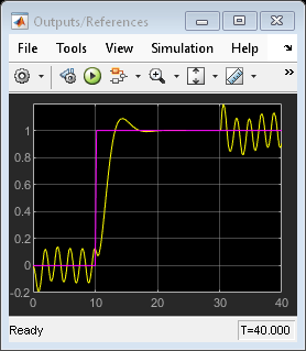
% Specify signals:
Tstop = 40;

% Reference signal: step change at time t=10
ref.time = 0:Ts:(Tstop+p*Ts);
ref.signals.values = double(ref.time>10)';

% Measured Disturbance Signal: step change at time t=30
md.time = ref.time;
md.signals.values = double(md.time>30)';
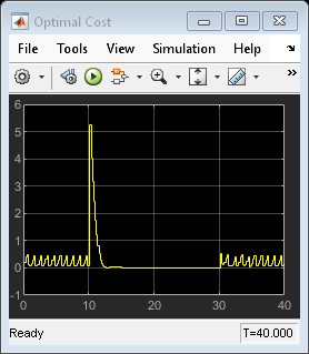
The relational operator block compares the calculated costs over the horizon, and its output signal is used to select the manipulated variable from the controller that has the least cost over the horizon.
Open and simulate the Simulink model:
mdl = 'mpc_optimalcost';
open_system(mdl);                     % Open Simulink(R) Model
sim(mdl,Tstop);                       % Start Simulation

% open Simulink scopes
open_system([mdl '/MV']);
open_system([mdl '/Optimal Cost']);
open_system([mdl '/Outputs//References']);
-->Converting model to discrete time.
-->Integrator added as output disturbance model for measured output #1.
-->"Model.Noise" is empty. Assuming white noise on each measured output.
-->Converting model to discrete time.
-->Integrator added as output disturbance model for measured output #1.
-->"Model.Noise" is empty. Assuming white noise on each measured output.
Note that:
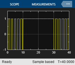
From time 0 to time 10, the control action keeps switching between MPC1 (-1) and MPC2 (+1). This is because the reference signal is 0 and it requires a controller output at 0 to reach steady state, which cannot be achieved with either MPC controller.
From time 10 to 30, MPC2 control output (+1) is chosen because the reference signal becomes +1 and it requires a controller output at +1 to reach steady state (plant gain is 1), which can be achieved by MPC2.
From time 30 to 40, control action starts switching again. This is because with the presence of measured disturbance (+1), MPC1 leads to a steady state of 0 and MPC2 leads to a steady state of +2, while the reference signal still requires +1.
Simulate Using MPCMOVE Command
Use mpcmove to perform step-by-step simulation and compute current MPC control action:
% Discrete-time dynamics
[Ad,Bd,Cd,Dd] = ssdata(c2d(plant,Ts));

% Number of simulation steps
Nsteps = round(Tstop/Ts);
Initialize matrices to store the simulation results
YY = zeros(Nsteps+1,1);
RR = zeros(Nsteps+1,1);
UU = zeros(Nsteps+1,1);
COST = zeros(Nsteps+1,1);

x = x0;                  % Initial plant state
xt1 = mpcstate(mpc1);    % Handle to initial state of controller #1
xt2 = mpcstate(mpc2);    % Handle to initial state of controller #2
Start simulation.
for td=0:Nsteps

    % Construct signals
    v = md.signals.values(td+1);
    r = ref.signals.values(td+1);

    % Plant equations: output update
    y = Cd*x + Dd(:,2)*v;

    % set option to return only the optimal cost in the solution structure
    options = mpcmoveopt;
    options.OnlyComputeCost = true;

    % Compute control moves ov both controllers
    [u1,Info1] = mpcmove(mpc1,xt1,y,r,v,options);
    [u2,Info2] = mpcmove(mpc2,xt2,y,r,v,options);

    % Compare the resulting optimal costs and choose the move
    % corresponding to the smallest cost value predicted over the horizon
    if Info1.Cost<=Info2.Cost
        u = u1;
        cost = Info1.Cost;
        % Update internal MPC state to the correct value
        xt2.Plant = xt1.Plant;
        xt2.Disturbance = xt1.Disturbance;
        xt2.LastMove = xt1.LastMove;
    else
        u = u2;
        cost = Info2.Cost;
        % Update internal MPC state to the correct value
        xt1.Plant = xt2.Plant;
        xt1.Disturbance = xt2.Disturbance;
        xt1.LastMove = xt2.LastMove;
    end

    % Store plant information
    YY(td+1) = y;
    RR(td+1) = r;
    UU(td+1) = u;
    COST(td+1) = cost;

    % Plant equations: state update
    x = Ad*x + Bd(:,1)*u + Bd(:,2)*v;
end
Plot the results of mpcmove to compare with the simulation results obtained in Simulink:
subplot(131)
plot((0:Nsteps)*Ts,[YY,RR]);                      % Plot output and reference signals
grid
title('OV and Reference')

subplot(132)
plot((0:Nsteps)*Ts,UU);                           % Plot manipulated variable
grid
title('MV')

subplot(133)
plot((0:Nsteps)*Ts,COST);                         % Plot optimal MPC value function
grid
title('Optimal cost')

The results are the same as the ones shown in the Simulink model scopes.
bdclose(mdl)
See Also
Functions
Objects
mpc|mpcstate|mpcmoveopt