Understanding Control Behavior by Examining Optimal Control Sequence
This example shows how to inspect the optimized sequence of manipulated variables computed by a model predictive controller at each sample time.
The plant is a double integrator subject to input saturation.
Design MPC Controller
The basic setup of the MPC controller includes:
A double integrator as the prediction model
A prediction horizon of
20A control horizon of
10Input constraints
-1 <= u(t) <= 1
Specify the MPC controller.
Ts = 0.1;
p = 20;
m = 10;
mpcobj = mpc(tf(1,[1 0 0]),Ts,p,m);
mpcobj.MV = struct('Min',-1,'Max',1);
nu = 1;
-->"Weights.ManipulatedVariables" is empty. Assuming default 0.00000.
-->"Weights.ManipulatedVariablesRate" is empty. Assuming default 0.10000.
-->"Weights.OutputVariables" is empty. Assuming default 1.00000.
Simulate Model in Simulink
To run this example, Simulink® is required.
if ~mpcchecktoolboxinstalled('simulink')
    disp('Simulink is required to run this example.')
    return
end
Open the Simulink model, and run the simulation.
mdl = 'mpc_sequence';
open_system(mdl)
sim(mdl)
-->Converting the "Model.Plant" property to state-space.
-->Converting model to discrete time.
   Assuming no disturbance added to measured output #1.
-->"Model.Noise" is empty. Assuming white noise on each measured output.


The MPC Controller block has an mv.seq output port, which is enabled by selecting the Optimal control sequence block parameter. This port outputs the optimal control sequence computed by the controller at each sample time. The output signal is an array with p+1 rows and Nmv columns, where p is prediction horizon and Nmv is the number of manipulated variables.
In a similar manner, the controller can output the optimal state sequence (x.seq) and the optimal output sequence (y.seq).
When the simulation stops, the To Workspace block connected to the mv.seq port exports this control sequence to the MATLAB® workspace, logging the data in the variable useq.
Analyze Optimal Control Sequences
Plot the optimal control sequence at specific time instants.
times = [0 0.2 1 2 2.1 2.2 3 3.5 5];
figure('Name','Optimal sequence history')
for t = 1:9
    ct = times(t)*10+1;
    subplot(3,3,t)
    h = stairs(0:p,useq.signals.values(ct,:));
    h.LineWidth = 1.5;
    hold on
    plot((0:p)+.5,useq.signals.values(ct,:),'*r')
    xlabel('prediction step')
    ylabel('u')
    title(sprintf('Sequence (t=%3.1f)',useq.time(ct)))
    grid
    axis([0 p -1.1 1.1])
    hold off
end

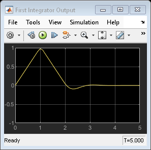
The MPC controller uses the first two seconds to bring the output very close to the set point. The controller output is at the upper limit (+1) for one second and switches to the lower limit (-1) for the next second, which is the best control strategy under the input constraints.
bdclose(mdl)