Boost Converter Controller Design Using Closed-Form Circuit Solution

Since R2026a

This example uses:

This example shows how to tune the gains of a digital controller to control the output voltage of a boost converter in the presence of load current disturbances.

Boost Converter Circuit

One of the challenges in designing the controller for a power train is obtaining the linear model at different operating conditions. Here we use the switched circuit analysis of the power train to generate the small signal model at diffgerent output voltages. These models are used to design the control using multi-objective tuning in Simulink Control Design™ functionality.

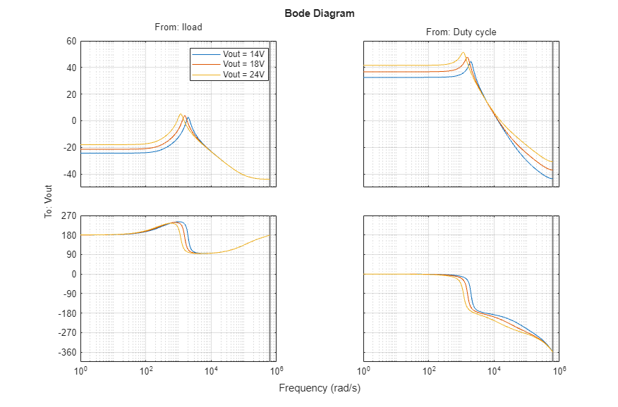
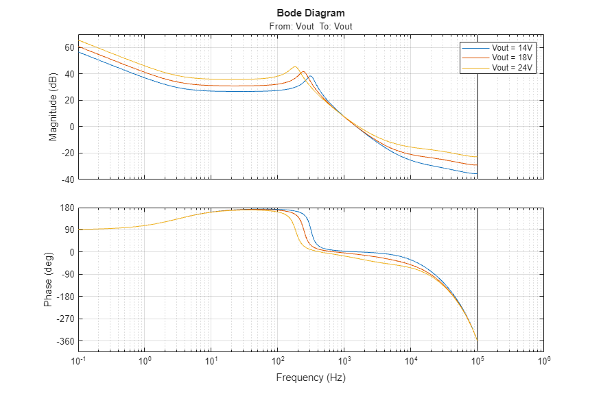
Use the cktconfig and cktoperpoint (add link) functions to compute the linear model as a state-space object in Control System Toolbox™. Visualizing the frequency response shows the variation in the dynamics of the switched circuit at output voltage levels of 14, 18 and 24 V.

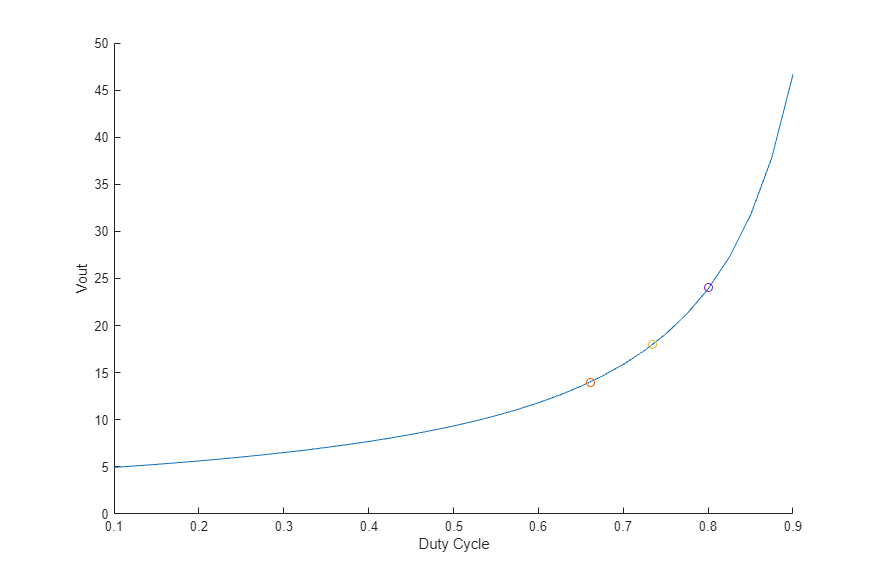
circuitModel = 'BoostConverterCircuit';
boostConverterCircuit = cktconfig(circuitModel,Ports={'cQ1','Vg','Iload','Vout','Iout','Ig'});

boostConverterCircuit.mdlwks.CircuitElementList(1).Value = 5;
boostConverterCircuit.CircuitDesignName='Boost SMPS';
boostConverterCircuit.BlockName='Power Train';
boostConverterCircuit.ConfigurationName='BoostSMPS';
boostConverterCircuit.OutputPort='Vout';
boostConverterCircuit.OutputValues=[14 18 24];
boostConverterCircuit.ControlVariable='Duty cycle';
boostConverterCircuit.DutyCycle=[0.1 0.9];
boostConverterCircuit.Frequency=200000;
boostConverterCircuit.PhaseOffsets='0';
boostConverterCircuit.PulseDuration='d';
boostConverterCircuit.WaveSamples=1024;

[~,~,~,boostConverterPlant,~] = cktoperpoint(boostConverterCircuit);

Visualize the Bode response for inputs ( 'Iload' and 'DutyCyle' ) to output ('Vout').

figure;
bp = bodeplot(boostConverterPlant(:,:,1),boostConverterPlant(:,:,2),boostConverterPlant(:,:,3));
bp.AxesStyle.GridVisible = 'on';
bp.Legend.Visible = 'on';
bp.Legend.String = ["Vout = 14V","Vout = 18V","Vout = 24V"];
bp.InputVisible = [false,true,true];
bp.OutputVisible = [true,false,false];

Boost Converter Control Model

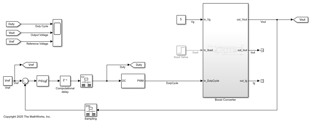
The 'BoostConverterControl.slx' model contains the runnable power train model using Simscape elements. A digital PID controller adjusts the PWM duty cycle, 'Duty', based on the voltage error between the reference and output values.

model = 'BoostConverterControl';
open_system(model);

The model uses the reference voltage and gains defined in the MATLAB workspace. This PID controller generates the duty cycle as a weighted combined effect of the instant voltage error, accumulated voltage error and the rate of change of voltage error.

Vref = 14; %#ok<*NASGU>
Kp = 0.5;
Ki = 10;
Kd = 1e-5;
N = 2e5;

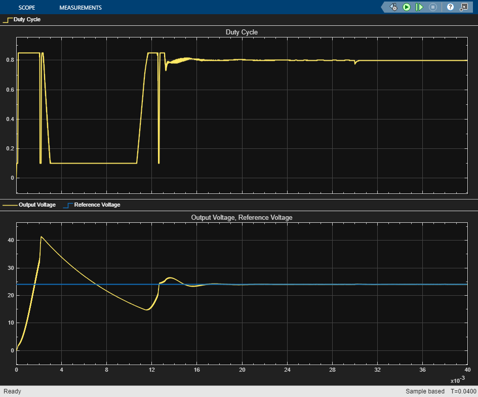
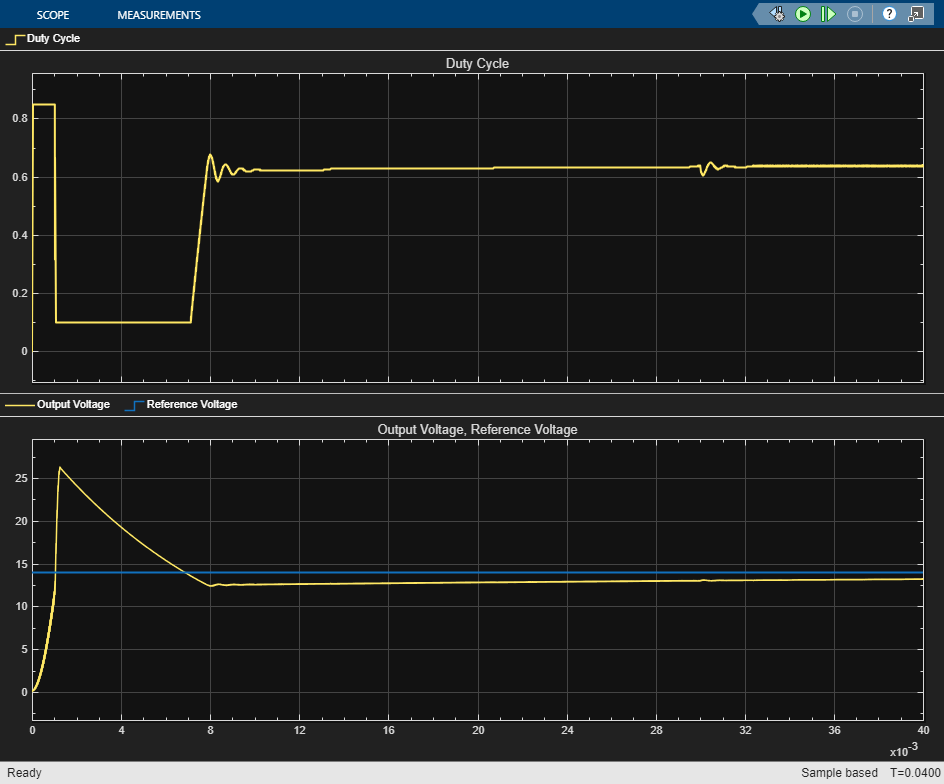
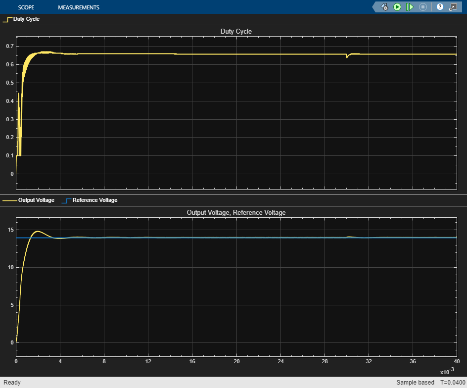
Simulating the model with the initial gains shows that even after the initial charge up phase of 8 ms it takes a long time for the output voltage to reach 14V. We can also observe oscillations when there are load current disturbances at 30 ms.

sim(model);

Custom Linearization for Boost Converter

The results from the "Boost Converter Circuit" section are used to provide a custom linearization via the Specify Individual Block Linearization approach for the Boost Converter subsystem. Simulink model linearization then uses the state-space model returned without having to replace the block.

The helper script, 'hGetLinearModelAtSpecifiedOutputVoltage.m' uses the commands to compute the state-space model for a specific output voltage. The variable 'Vout' is defined in the MATLAB workspace. Also note that the PWM subsystem also needs a custom linearization that represents the block as static gain of 1.

Vout = 14;
%<<../SpecifyBlockLinearization.png>>

Create an slTuner object based on the model, tunable block and signals of interest. Also define parameters that are used to linearize at different output voltages at a sample time of 5e-6 seconds.

tunableBlock = [model,'/PID Controller'];
signalsOfInterest = {'Vref','Vg','Iload','DutyCycle','Vout','Iout','Ig'};
ST0 = slTuner(model,tunableBlock,signalsOfInterest);
ST0.Parameters = struct(Name='Vout',Value=[14 18 24]);
ST0.Options.SampleTime = 5e-6;

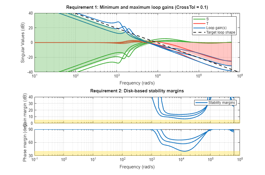
Analyze the loop response at 'Vout', with the initial, untuned controller gains. Observe that the bandwidth is low, with resonant peaks leading to oscillations. We can also see that the phase and gain margins are not enough to provide robustness against disturbances.

openLoopSystem = getLoopTransfer(ST0,'Vout');
figure;
bp = bodeplot(openLoopSystem(:,:,1),openLoopSystem(:,:,2),openLoopSystem(:,:,3));
bp.AxesStyle.GridVisible = 'on';
bp.FrequencyUnit = 'Hz';
bp.Legend.Visible = 'on';
bp.Legend.String = ["Vout = 14V","Vout = 18V","Vout = 24V"];

Tune PID Controller

The PID Controller block is tuned by first defining TuningGoal requirements for loop bandwidth and margins and then using systune, a fixed structure controller tuning method, to compute the tunable gains.

Use TuningGoal.LoopShape to specify a target bandwidth of '1.5 KHz' and TuningGoal.Margins to specify phase and gain margins of '40 degrees' and '5 dB' respectively.

loopShapeTG = TuningGoal.LoopShape('Vout',2*pi*1.5e3);
marginTG = TuningGoal.Margins('Vout',5,40);

Use systune to compute the tunable parameters of the PID block, specifying the loop shape goal as a soft requirement and the margins as a hard requirement. The 'Hard' objective value of less than 1 and the 'Soft' objective value of between 1 and 2 show that the optimization found the minimum objective solution for the loop shape while satisfying the margin requirements.

ST = systune(ST0,loopShapeTG,marginTG);

Final: Soft = 1.92, Hard = 0.99981, Iterations = 175

Use viewGoal to visualize the tuned loop against the requirements, showing the improvement in the bandwidth and the margins.

figure;
viewGoal([loopShapeTG,marginTG],ST);

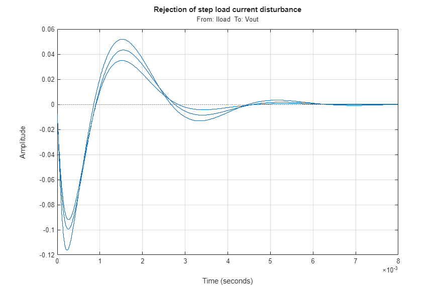
Visualize the step response of the load current input, 'Iload', to the output voltage, 'Vout', to observe the rejection of load disturbances. The peak response to the disturbance is low and the transients settle to zero within 6 ms.

loadDisturbanceSys = getIOTransfer(ST,'Iload','Vout');
figure;
sp = stepplot(loadDisturbanceSys);
sp.Title.String = "Rejection of step load current disturbance";
sp.AxesStyle.GridVisible = 'on';

Validate Controller Design

The tuned values are stored in the MATLAB workspace and the model is simulated again to observe the results.

tunedController = getBlockValue(ST,'PID Controller');
Kp = tunedController.Kp;
Ki = tunedController.Ki;
Kd = tunedController.Kd;
N = 1/tunedController.Tf;

sim(model);

Change the reference voltage to 24V to validate the performance of the controller at a different operating condition. Note that while the initial charge up takes longer for the increased reference voltage, the time to settle, steady state and disturbance rejection characteristics is similar to that of 14 V.

Vref = 24;
sim(model);