Plot the Solution in the PDE Modeler App
To plot a solution property, use the Plot menu. Use the Plot Selection dialog box to select which property to plot, which plot style to use, and several other plot parameters. If you have recorded a movie (animation) of the solution, you can export it to the workspace.
To open the Plot Selection dialog box, select
Parameters from the Plot menu or
click the ![]() button.
button.

Parameters opens a dialog box containing options controlling the plotting and visualization.
The upper part of the dialog box contains four columns:
Plot type (far left) contains a row of six different plot types, which can be used for visualization:
Color. Visualization of a scalar property using colored surface objects.
Contour. Visualization of a scalar property using colored contour lines. The contour lines can also enhance the color visualization when both plot types (Color and Contour) are checked. The contour lines are then drawn in black.
Arrows. Visualization of a vector property using arrows.
Deformed mesh. Visualization of a vector property by deforming the mesh using the vector property. The deformation is automatically scaled to 10% of the problem domain. This plot type is primarily intended for visualizing x- and y-displacements (u and v) for problems in structural mechanics. If no other plot type is selected, the deformed triangular mesh is displayed.
Height (3-D plot). Visualization of a scalar property using height (z-axis) in a 3-D plot. 3-D plots are plotted in separate figure windows. If the Color and Contour plot types are not used, the 3-D plot is simply a mesh plot. You can visualize another scalar property simultaneously using Color and/or Contour, which results in a 3-D surface or contour plot.
Animation. Animation of time-dependent solutions to parabolic and hyperbolic problems. If you select this option, the solution is recorded and then animated in a separate figure window using the MATLAB®
moviefunction.
A color bar is added to the plots to map the colors in the plot to the magnitude of the property that is represented using color or contour lines.
Property contains four pop-up menus containing lists of properties that are available for plotting using the corresponding plot type. From the first pop-up menu you control the property that is visualized using color and/or contour lines. The second and third pop-up menus contain vector valued properties for visualization using arrows and deformed mesh, respectively. From the fourth pop-up menu, finally, you control which scalar property to visualize using z-height in a 3-D plot. The lists of properties are dependent on the current application mode. For the generic scalar mode, you can select the following scalar properties:
u. The solution itself.
abs(grad(u)). The absolute value of ∇u, evaluated at the center of each triangle.
abs(c*grad(u)). The absolute value of c · ∇u, evaluated at the center of each triangle.
user entry. A MATLAB expression returning a vector of data defined on the nodes or the triangles of the current triangular mesh. The solution
u, its derivativesuxanduy, the x and y components of c · ∇u,cuxandcuy, andxandyare all available in the local workspace. You enter the expression into the edit box to the right of the Property pop-up menu in the User entry column.Examples:
u.*u, x+y
The vector property pop-up menus contain the following properties in the generic scalar case:
-grad(u). The negative gradient of u, –∇u.
-c*grad(u). c times the negative gradient of u, –c · ∇u.
user entry. A MATLAB expression
[px;
py]
returning a 2-by-ntri matrix of data defined on the triangles of the current triangular mesh (ntri is the number of triangles in the current mesh). The solutionu, its derivativesuxanduy, the x and y components of c · ∇u,cuxandcuy, andxandyare all available in the local workspace. Data defined on the nodes is interpolated to triangle centers. You enter the expression into the edit field to the right of the Property pop-up menu in the User entry column.Examples:
[ux;uy], [x;y]
For the generic system case, the properties available for visualization using color, contour lines, or z-height are u, v, abs(u,v), and a user entry. For visualization using arrows or a deformed mesh, you can choose (u,v) or a user entry. For applications in structural mechanics, u and v are the x- and y-displacements, respectively.
The variables available in the local workspace for a user entered
expression are the same for all scalar and system modes (the solution
is always referred to as u and, in the system case, v).
User entry contains four edit fields where you can enter your own expression, if you select the user entry property from the corresponding pop-up menu to the left of the edit fields. If the user entry property is not selected, the corresponding edit field is disabled.
Plot style contains three pop-up menus from which you can control the plot style for the color, arrow, and height plot types respectively. The available plot styles for color surface plots are
Interpolated shading. A surface plot using the selected colormap and interpolated shading, i.e., each triangular area is colored using a linear, interpolated shading (the default).
Flat shading. A surface plot using the selected colormap and flat shading, i.e., each triangular area is colored using a constant color.
You can use two different arrow plot styles:
Proportional. The length of the arrow corresponds to the magnitude of the property that you visualize (the default).
Normalized. The lengths of all arrows are normalized, i.e., all arrows have the same length. This is useful when you are interested in the direction of the vector field. The direction is clearly visible even in areas where the magnitude of the field is very small.
For height (3-D plots), the available plot styles are:
Continuous. Produces a “smooth” continuous plot by interpolating data from triangle midpoints to the mesh nodes (the default).
Discontinuous. Produces a discontinuous plot where data and z-height are constant on each triangle.
A total of three properties of the solution—two scalar properties and one vector
field—can be visualized simultaneously. If the Height (3-D plot)
option is turned off, the solution plot is a 2-D plot and is plotted in the main axes of the
PDE Modeler app. If the Height (3-D plot) option is used, the solution
plot is a 3-D plot in a separate figure window. If possible, the 3-D plot uses an existing
figure window. If you would like to plot in a new figure window, simply type
figure at the MATLAB command line.
Additional Plot Control Options
In the middle of the dialog box are a number of additional plot control options:
Plot in x-y grid. If you select this option, the solution is converted from the original triangular grid to a rectangular x-y grid. This is especially useful for animations since it speeds up the process of recording the movie frames significantly.
Show mesh. In the surface plots, the mesh is plotted using black color if you select this option. By default, the mesh is hidden.
Contour plot levels. For contour plots, the number of level curves, e.g.,
15or20can be entered. Alternatively, you can enter a MATLAB vector of levels. The curves of the contour plot are then drawn at those levels. The default is 20 contour level curves.Examples:
[0:100:1000],logspace(-1,1,30)Colormap. Using the Colormap pop-up menu, you can select from a number of different color maps:
cool,gray,bone,pink,copper,hot,jet,hsv,prism, andparula.Plot solution automatically. This option is normally selected. If turned off, there will not be a display of a plot of the solution immediately upon solving the PDE. The new solution, however, can be plotted using this dialog box.
For the parabolic and hyperbolic PDEs, the bottom right portion of the Plot Selection dialog box contains the Time for plot parameter.
Time for plot. A pop-up menu allows you to select which of the solutions to plot by selecting the corresponding time. By default, the last solution is plotted.
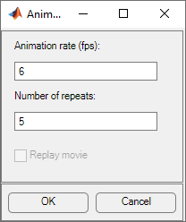
Also, the Animation plot type is enabled. In its property field you find an Options button. If you press it, an additional dialog box appears. It contains parameters that control the animation:
Animation rate (fps). For the animation, this parameter controls the speed of the movie in frames per second (fps).
Number of repeats. The number of times the movie is played.
Replay movie. If you select this option, the current movie is replayed without rerecording the movie frames. If there is no current movie, this option is disabled.
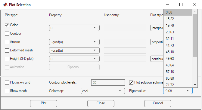
For eigenvalue problems, the bottom right part of the dialog box contains a drop-down menu with all eigenvalues. The plotted solution is the eigenvector associated with the selected eigenvalue. By default, the smallest eigenvalue is selected.
You can rotate the 3-D plots by clicking the plot and, while keeping the mouse button down, moving the mouse. For guidance, a surrounding box appears. When you release the mouse, the plot is redrawn using the new viewpoint. Initially, the solution is plotted using -37.5 degrees horizontal rotation and 30 degrees elevation.
If you click the Plot button, the solution is plotted immediately using the current plot setup. If there is no current solution available, the PDE is first solved. The new solution is then plotted. The dialog box remains on the screen.
If you click the Done button, the dialog box is closed. The current setup is saved but no additional plotting takes place.
If you click the Cancel button, the dialog box is closed. The setup remains unchanged since the last plot.
Tooltip Displays for Mesh and Plots
In mesh mode, you can use the mouse to display the node number and the triangle number at the position where you click. Press the left mouse button to display the node number on the information line. Use the left mouse button and the Shift key to display the triangle number on the information line.
In plot mode, you can use the mouse to display the numerical value of the plotted property at the position where you click. Press the left mouse button to display the triangle number and the value of the plotted property on the information line.
The information remains on the information line until you release the mouse button.