Joint Radar-Communication Using PMCW and OFDM Waveforms
This example shows how to model a joint radar-communication (JRC) system using the Phase Array System Toolbox. Two modulation schemes for combining radar and communication signals are presented. The first scheme uses the phase-modulated continuous wave (PMCW) waveform. The second scheme uses the orthogonal frequency division multiplexing (OFDM) waveform. For each modulation scheme the example shows how to process the received signal by both the radar and the communication receivers.
JRC System Parameters
JRC is one of many different radar and communication coexistence strategies. Such strategies have emerged recently as a response to an increasingly congested frequency spectrum and a demand of radar and communication systems for a large bandwidth. In a JRC system both the radar and the communication share the same platform and have a common transmit waveform. This example shows two approaches to utilizing a single waveform for both functions. The first approach uses PMCW. Such a JRC system can be considered as radar-centric, since PMCW is a waveform tailored to radar applications. The second approach uses OFDM. This approach is communication-centric since a communication waveform is used to perform the radar function.
Consider a JRC system that operates at a carrier frequency of 24 GHz and has a bandwidth of 100 MHz.
% Set the random number generator for reproducibility
rng('default');

fc = 24e9;                              % Carrier frequency (Hz)
B = 100e6;                              % Bandwidth (Hz)
Set the peak transmit power to 10 mW and the transmit antenna gain to 20 dB.
Pt = 0.01;                              % Peak power (W)
Gtx = 20;                               % Tx antenna gain (dB)
Let the JRC transmitter and the radar receiver be colocated at the origin. Create a phased.Platform object to represent the JRC system.
jrcpos = [0; 0; 0];                     % JRC position
jrcvel = [0; 0; 0];                     % JRC velocity

jrcmotion = phased.Platform('InitialPosition', jrcpos, 'Velocity', jrcvel);
Assume the radar receiver has the following parameters.
Grx = 20;                               % Radar Rx antenna gain (dB)
NF = 2.9;                               % Noise figure (dB)
Tref = 290;                             % Reference temperature (K)
Let the maximum range of interest and the maximum observed relative velocity be 200 m and 60 m/s respectively.
Rmax = 200;                             % Maximum range of interest
vrelmax = 60;                           % Maximum relative velocity
Consider a scenario with three moving radar targets and a single downlink user. Create a phased.Platform object to represent moving targets and a phased.RadarTarget object to represent the target's radar cross sections (RCS).
tgtpos = [110 45 80; -10 5 -4; 0 0 0];  % Target positions
tgtvel = [-15 40 -32; 0 0 0; 0 0 0];    % Target velocities
tgtmotion = phased.Platform('InitialPosition', tgtpos, 'Velocity', tgtvel);

tgtrcs = [4.7 3.1 2.3];                 % Target RCS
target = phased.RadarTarget('Model', 'Swerling1', 'MeanRCS', tgtrcs, 'OperatingFrequency', fc);
Create a position vector to represent the position of the downlink user.
userpos = [100; 20; 0]; % Downlink user position Visualize the JRC scenario using helperPlotJRCScenario helper function.
helperPlotJRCScenario(jrcpos, tgtpos, userpos, tgtvel);

JRC System Using a PMCW Waveform
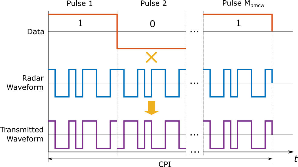
The first modulation scheme considered in this example uses a PMCW waveform. A PMCW radar repeatedly transmits a selected phase-coded sequence. The duration of the transmitted sequence is called a modulation period. Since the duty cycle of a PMCW radar is equal to one, the next modulation period starts right after the previous.
This example uses a maximum length pseudo-random binary sequence (PRBS) also frequently referred to as an m-sequence. Maximum length sequences have low autocorrelation sidelobes that result in a good range estimation performance. The communication data is modulated on top of the radar waveform such that each modulation period carries a single bit. This is achieved by simply multiplying the entire modulation period by the corresponding BPSK symbol.
Using the helperMLS helper function create a PRBS.
% Generate an m-sequence. The sequence lengths has to be 2^p-1, where p is
% an integer.
p = 8;
prbs = helperMLS(p);
Nprbs = numel(prbs);                    % Number of chips in PRBS
Given that the chip duration of a phase-modulated waveform is an inverse of the total bandwidth, compute the modulation period.
Tchip = 1/B;                             % Chip duration
Tprbs = Nprbs * Tchip;                   % Modulation period
Generate the communication data to be transmitted. Encode the generated data bits using the BPSK modulation.
Mpmcw = 256;                             % Number of transmitted data bits
dataTx = randi([0, 1], [Mpmcw 1]);       % Binary data
bpskTx = pskmod(dataTx, 2);              % BPSK symbols
Since the communication channel is unknown, the JRC system must perform channel sounding. One way to do it is to send out a single period of the PRBS sequence unmodulated with the communication data. Thus, a transmission of one data bit would require transmitting the PRBS sequence twice. The first time to sound the channel, the second time to transmit the data. Create the PMCW waveform by stacking two modulation periods together, the first period is just the generated PRBS and the second period is the generated PRBS multiplied by the corresponding BPSK symbol.
% Transmit waveform
xpmcw = [prbs * ones(1, Mpmcw); prbs * bpskTx.'];
Thus, the duration of one PMCW block is twice the modulation period.
Tpmcw = 2*Tprbs;
The block duration can be longer if the same data symbol has to be repeated multiple times in order to improve the signal-to-noise ratio (SNR) by integrating multiple periods at the receiver.
Assume that the coherent processing interval is long enough to coherently process Mpmcw blocks. Compute the duration of a single PMCW frame that carries Mpmcw data bits.
Tpmcw*Mpmcw
ans =
0.0013
Radar Signal Simulation and Processing
This section of the example shows how to simulate the radar sensing part of the JRC system with the PMCW waveform. First, generate received PMCW blocks.
% Set the sample rate equal to the bandwidth
fs = B;

% Setup the transmitter and the radiator
transmitter = phased.Transmitter('Gain', Gtx, 'PeakPower', Pt);

% Assume the JRC is using an isotropic antenna
ant = phased.IsotropicAntennaElement;
radiator = phased.Radiator('Sensor', ant, 'OperatingFrequency', fc);

% Setup the collector and the receiver
collector = phased.Collector('Sensor', ant, 'OperatingFrequency', fc);
receiver = phased.ReceiverPreamp('SampleRate', fs, 'Gain', Grx, 'NoiseFigure', NF, 'ReferenceTemperature', Tref);

% Setup a free space channel to model the JRC signal propagation from the
% transmitter to the targets and back to the radar receiver
radarChannel = phased.FreeSpace('SampleRate', fs, 'TwoWayPropagation', true, 'OperatingFrequency', fc);

% Preallocate space for the signal received by the radar receiver
ypmcwr = zeros(size(xpmcw));

% Transmit one PMCW block at a time assuming that all Mpmcw blocks are
% transmitted within a single CPI
for m = 1:Mpmcw
    % Update sensor and target positions
    [jrcpos, jrcvel] = jrcmotion(Tpmcw);
    [tgtpos, tgtvel] = tgtmotion(Tpmcw);

    % Calculate the target angles as seen from the transmit array
    [tgtrng, tgtang] = rangeangle(tgtpos, jrcpos);

    % Transmit signal
    txsig = transmitter(xpmcw(:, m));

    % Radiate signal towards the targets
    radtxsig = radiator(txsig, tgtang);

    % Apply free space channel propagation effects
    chansig = radarChannel(radtxsig, jrcpos, tgtpos, jrcvel, tgtvel);

    % Reflect signal off the targets
    tgtsig = target(chansig, false);

    % Receive target returns at the receive array
    rxsig = collector(tgtsig, tgtang);

    % Add thermal noise at the receiver
    ypmcwr(:, m) = receiver(rxsig);
end
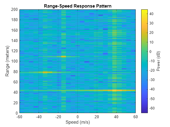
Now the received signals can be processed to obtain estimates of the targets ranges and velocities. The following diagram shows the signal processing steps needed to compute the range-Doppler map.

Start by removing the communication data. Multiply the modulation periods that carry the data by the corresponding BPSK symbols.
ypmcwr1 = ypmcwr(Nprbs+1:end, :) .* (bpskTx.');
The modulation period used for the communication channel sounding can be integrated with the modulation period that carried the data.
ypmcwr1 = ypmcwr1 + ypmcwr(1:Nprbs, :);
It is more computationally efficient to perform matched filtering in the frequency domain. First, compute the frequency domain representation of the integrated signal then, multiply the result by the complex-conjugate version of the DFT of the used PRBS.
% Frequency-domain matched filtering
Ypmcwr = fft(ypmcwr1);
Sprbs = fft(prbs);
Zpmcwr = Ypmcwr .* conj(Sprbs);
Use phased.RangeDopplerResponse to compute and plot the range-Doppler map.
% Range-Doppler response object computes DFT in the slow-time domain and
% then IDFT in the fast-time domain to obtain the range-Doppler map
rdr = phased.RangeDopplerResponse('RangeMethod', 'FFT', 'SampleRate', fs, 'SweepSlope', -B/Tprbs,...
    'DopplerOutput', 'Speed', 'OperatingFrequency', fc, 'PRFSource', 'Property', 'PRF', 1/Tpmcw,...
    'ReferenceRangeCentered', false);

figure;
plotResponse(rdr, Zpmcwr, 'Unit', 'db');
xlim([-vrelmax vrelmax]);
ylim([0 Rmax]);
Communication Signal Simulation and Processing
This example uses a stochastic Rician channel model to simulate the propagation of the JRC signal from the transmitter to the downlink receiver. Create a communication channel object and pass the PMCW signal through the channel.
% Line-of-sight between the JRC transmitter and the downlink user
dlos = vecnorm(jrcpos - userpos);
taulos = dlos/physconst('LightSpeed');

% Delays and gains due to different path in the communication channel
pathDelays = taulos * [1 1.6 1.1 1.45] - taulos;
averagePathGains = [0 -1 2 -1.5];

% Maximum two-way Doppler shift
fdmax = 2 * speed2dop(vrelmax, freq2wavelen(fc));
commChannel = comm.RicianChannel('PathGainsOutputPort', true, 'DirectPathDopplerShift', 0,...
    'MaximumDopplerShift', fdmax/2, 'PathDelays', pathDelays, 'AveragePathGains', averagePathGains, ...
    'SampleRate', fs);

% Pass the transmitted signal through the channel
ypmcwc = commChannel(xpmcw(:));
For simplicity, model the downlink receiver using additive gaussian noise and assuming that the signal-to-noise ratio (SNR) is 40 dB.
SNRu = 40;                               % SNR at the downlink user's receiver
ypmcwc = awgn(ypmcwc, SNRu, "measured");
ypmcwc = reshape(ypmcwc, 2*Nprbs, []);
Use the first PRBS repetition in each PMCW block to estimate the channel frequency response.
ysound = ypmcwc(1:Nprbs, :);
Hpmcw = fft(ysound)./Sprbs;
Once the channel estimates are available, the received signal can be processed to extract the user data. The diagram below show the required processing steps.

Since a radar waveform is used to carry the user data, the matched filtering is the first step in the demodulation process. Perform matched filtering in the frequency domain.
% Compute the frequency domain representation of the received signal
Ypmcwc = fft(ypmcwc(Nprbs + 1:end, :));

% Multiply by the complex-conjugate version of the DFT of the used PRBS
Zpmcwc = Ypmcwc .* conj(Sprbs);
Multiply the frequency representation of the matched filtered signal by the inverse of the estimated channel frequency response to remove the channel effects.
Zpmcwc = Zpmcwc./Hpmcw;
Demodulate the signal to first obtain the BPSK symbols and then the binary data.
zpmcwc = ifft(Zpmcwc);

[~, idx] = max(abs(zpmcwc), [], 'linear');
bpskRx = zpmcwc(idx).';
bpskRx = bpskRx./Nprbs;
dataRx = pskdemod(bpskRx, 2);

refconst = pskmod([0 1], 2);
constellationDiagram = comm.ConstellationDiagram('NumInputPorts', 1, ...
    'ReferenceConstellation', refconst, 'ChannelNames', {'Received PSK Symbols'});
constellationDiagram(bpskRx(:));

Compute the bit error rate.
[numErr, ratio] = biterr(dataTx, dataRx)
numErr =
0
ratio =
0
JRC System Using an OFDM Waveform
OFDM is a second modulation scheme considered in this example. OFDM signals are widely used for wireless communication. OFDM is a multicarrier signal composed of a set of orthogonal complex exponentials known as subcarriers. The complex amplitude of each subcarrier can be used to carry communication data allowing for a high data rate. OFDM waveforms were also noted to exhibit Doppler tolerance and a lack of range-Doppler coupling. These OFDM features are attractive to radar applications. This section of the example shows how to use an OFDM waveform to perform both the radar sensing and communication.
Let the number of OFDM subcarriers be 1024. Compute the subcarrier separation given that all subcarriers must be equally spaced in frequency.
Nsc = 1024;                              % Number of subcarriers
df = B/Nsc;                              % Separation between OFDM subcarriers
Tsym = 1/df;                             % OFDM symbol duration
According to the OFDM system design rules, the subcarrier spacing must be at least ten times larger than the maximum Doppler shift experienced by the signal. This is required to ensure the orthogonality of the subcarrier. Verify that this condition is met for the scenario considered in this example.
df > 10*fdmax
ans = logical
   1
In order to avoid intersymbol interference, the OFDM symbols are prepended with cyclic prefix. Compute the cyclic prefix duration based on the maximum range of interest.
Tcp = range2time(Rmax);                  % Duration of the cyclic prefix (CP)
Ncp = ceil(fs*Tcp);                      % Length of the CP in samples
Tcp = Ncp/fs;                            % Adjust duration of the CP to have an integer number of samples

Tofdm = Tsym + Tcp;                      % OFDM symbol duration with CP
Nofdm = Nsc + Ncp;                       % Number of samples in one OFDM symbol
Designate some of the subcarriers to act as guard bands.
nullIdx = [1:9 (Nsc/2+1) (Nsc-8:Nsc)]';  % Guard bands and DC subcarrier
Nscd = Nsc-length(nullIdx);              % Number of data subcarriers
Generate binary data to be transmitted. Since each OFDM subcarrier can carry a complex data symbol, the generated binary data first must be modulated. Use QAM-modulation to modulate the generated binary data. Finally, OFDM-modulate the QAM-modulated symbols.
bps = 6;                                 % Bits per QAM symbol (and OFDM data subcarrier)
K = 2^bps;                               % Modulation order
Mofdm = 128;                             % Number of transmitted OFDM symbols
dataTx = randi([0,1], [Nscd*bps Mofdm]);
qamTx = qammod(dataTx, K, 'InputType', 'bit', 'UnitAveragePower', true);
ofdmTx = ofdmmod(qamTx, Nsc, Ncp, nullIdx);
Assume that the coherent processing interval is long enough to coherently process Mofdm symbols. Compute the duration of a single OFDM frame and a total number of data bits in one frame.
Tofdm*Mofdm % Frame duration (s)ans = 0.0015
Nscd*bps*Mofdm % Total number of bitsans = 771840
Notice that the OFDM frame duration is close to the PMCW frame duration, however the total number of transmitted bits is larger by several orders of magnitude.
Radar Signal Simulation and Processing
Use the same system as in the PMCW case to simulate transmission of the OFDM signal by the JRC and the reception of the target returns by the radar receiver.
xofdm = reshape(ofdmTx, Nofdm, Mofdm);

% OFDM waveform is not a constant modulus waveform. The generated OFDM
% samples have power much less than one. To fully utilize the available
% transmit power, normalize the waveform such that the sample with the
% largest power had power of one.
xofdm = xofdm/max(sqrt(abs(xofdm).^2), [], 'all');

% Preallocate space for the signal received by the radar receiver
yofdmr = zeros(size(xofdm));

% Reset the platform objects representing the JRC and the targets before
% running the simulation
reset(jrcmotion);
reset(tgtmotion);

% Transmit one OFDM symbol at a time assuming that all Mofdm symbols are
% transmitted within a single CPI
for m = 1:Mofdm
    % Update sensor and target positions
    [jrcpos, jrcvel] = jrcmotion(Tofdm);
    [tgtpos, tgtvel] = tgtmotion(Tofdm);

    % Calculate the target angles as seen from the transmit array
    [tgtrng, tgtang] = rangeangle(tgtpos, jrcpos);

    % Transmit signal
    txsig = transmitter(xofdm(:, m));

    % Radiate signal towards the targets
    radtxsig = radiator(txsig, tgtang);

    % Apply free space channel propagation effects
    chansig = radarChannel(radtxsig, jrcpos, tgtpos, jrcvel, tgtvel);

    % Reflect signal off the targets
    tgtsig = target(chansig, false);

    % Receive target returns at the receive array
    rxsig = collector(tgtsig, tgtang);

    % Add thermal noise at the receiver
    yofdmr(:, m) = receiver(rxsig);
end
Process the target returns to obtain a range-Doppler map. The signal processing steps are shown in the block diagram.

Remove the cyclic prefix and compute the DFT in the fast-time domain using the ofdmdemod function.
yofdmr1 = reshape(yofdmr, Nofdm*Mofdm, 1);

% Demodulate the received OFDM signal (compute DFT)
Yofdmr = ofdmdemod(yofdmr1, Nsc, Ncp, Ncp, nullIdx);
The complex amplitudes of the subcarriers that comprise the received OFDM signal are the transmitted QAM symbols. Therefore, to remove the communication data divide the DFT of the received signal by the transmitted QAM symbols.
Zofdmr = Yofdmr./qamTx;
Use phased.RangeDopplerResponse to compute and plot the range-Doppler map.
% Range-Doppler response object computes DFT in the slow-time domain and
% then IDFT in the fast-time domain to obtain the range-Doppler map
rdr = phased.RangeDopplerResponse('RangeMethod', 'FFT', 'SampleRate', fs, 'SweepSlope', -B/Tofdm,...
    'DopplerOutput', 'Speed', 'OperatingFrequency', fc, 'PRFSource', 'Property', 'PRF', 1/Tofdm, ...
    'ReferenceRangeCentered', false);

figure;
plotResponse(rdr, Zofdmr, 'Unit', 'db');
xlim([-vrelmax vrelmax]);
ylim([0 Rmax]);

Communication Signal Simulation and Processing
Use the same stochastic Rician channel model as in the case of the PMCW to model the signal propagation from the JRC transmitter to the downlink user.
[yofdmc, pathGains] = commChannel(ofdmTx);
Add the receiver noise.
yofdmc = awgn(yofdmc, SNRu, "measured");Compute the OFDM channel response to perform channel equalization.
channelInfo = info(commChannel);
pathFilters = channelInfo.ChannelFilterCoefficients;
toffset = channelInfo.ChannelFilterDelay;
Hofdm = ofdmChannelResponse(pathGains, pathFilters, Nsc, Ncp, ...
    setdiff(1:Nsc, nullIdx), toffset);
Perform demodulation and equalization. The block diagram of the processing steps is shown below.

zeropadding = zeros(toffset, 1);
ofdmRx = [yofdmc(toffset+1:end,:); zeropadding];

qamRx = ofdmdemod(ofdmRx, Nsc, Ncp, Ncp/2, nullIdx);
qamEq = ofdmEqualize(qamRx, Hofdm(:), 'Algorithm', 'zf');
Demodulate the QAM symbols to obtain the received binary data.
dataRx = qamdemod(qamEq, K, 'OutputType', 'bit', 'UnitAveragePower', true);

refconst = qammod(0:K-1, K, 'UnitAveragePower', true);
constellationDiagram = comm.ConstellationDiagram('NumInputPorts', 1, ...
    'ReferenceConstellation', refconst, 'ChannelNames', {'Received QAM Symbols'});

% Show QAM data symbols comprising the first 10 received OFDM symbols
constellationDiagram(qamEq(1:Nscd*10).');

Compute the bit error rate.
[numErr,ratio] = biterr(dataTx, dataRx)
numErr =
14754
ratio =
0.0191
Conclusions
This example simulates a JRC system using two different modulation schemes for generating a transmit waveform: PMCW and OFDM. The transmit waveforms are generated such that they can be used to sense radar targets and to carry communication data. The example shows how to simulate transmission, propagation, and reception of these waveforms by the radar receiver and by the downlink user. For each modulation scheme the example shows how to perform radar signal processing to obtain a range-Doppler map of the observed scenario. The example also shows how to process the received signal at the downlink receiver to obtain the transmitted communication data.
References
Sturm, Christian, and Werner Wiesbeck. "Waveform design and signal processing aspects for fusion of wireless communications and radar sensing." Proceedings of the IEEE 99, no. 7 (2011): 1236-1259.
de Oliveira, Lucas Giroto, Benjamin Nuss, Mohamad Basim Alabd, Axel Diewald, Mario Pauli, and Thomas Zwick. "Joint radar-communication systems: Modulation schemes and system design." IEEE Transactions on Microwave Theory and Techniques 70, no. 3 (2021): 1521-1551.
Supporting Functions
function seq = helperMLS(p)
% Generate a pseudorandom sequence of length N=2^p-1, where p is an
% integer. The sequence is generated using shift registers. The feedback
% coefficients for the registers are obtained from the coefficients of an
% irreducible, primitive polynomial in GF(2p).

    pol = gfprimdf(p, 2);
    seq = zeros(2^p - 1, 1);
    seq(1:p) = randi([0 1], p, 1);

    for i = (p + 1):(2^p - 1)
        seq(i) = mod(-pol(1:p)*seq(i-p : i-1), 2);
    end

    seq(seq == 0) = -1;
end