Validating Passive Radar Model with Real World Data

Since R2026a

Passive radar systems use existing transmissions to detect and track objects, offering unique advantages in stealth, spectral efficiency and hardware simplicity. This example demonstrates how to use the Phased Array System Toolbox and the Radar Toolbox with the ADALM-PHASER (CN0566) board to implement and validate a passive radar workflow.

In this example, you will:

• Set up and run a simulation of a passive receiver, including realistic RF hardware impairments.

• Simulate varying conditions by running the scenario multiple times with different parameter settings.

• Implement a bistatic radar signal processing workflow on simulated data.

• Validate the workflow with real-world data.

• Compare signal-to-interference-plus-noise ratio (SINR) between simulation and measurement to demonstrate that the simulation accurately reflects real-world performance.

This example provides a practical, end-to-end workflow for passive radar development, from simulation through to real data validation.

The following video shows the results of the passive radar processing routine discussed in this example:

The data collection routines and instructions for the passive radar shown above can be found in the Phaser (CN0566) Control With MATLAB repository.

For this example, a single data frame from the video is analyzed.

Passive Radar Scenario

The following schematic demonstrates a generic passive radar scenario similar to the one that we will analyze in this example:

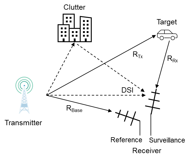
The transmitter in this scenario is radiating continuously. The receiver has two separate receive channels. The reference channel antenna points towards the transmitter location and the surveillance channel antenna points towards the surveillance area containing targets.

The real-world data collection was done in a parking lot, with a target vehicle driving between rows of parked cars. We create a radar scenario to model the location of the transmitter, receiver, target vehicle, and parked vehicles.

rng("default");
scene = helperSetupScene();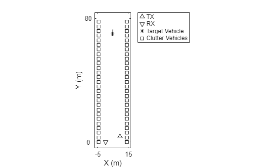

For more information on creating a radar scenario with bistatic geometry, refer to Cooperative Bistatic Radar I/Q Simulation and Processing (Radar Toolbox).

System Model Definition

In this section we discuss the hardware that will be used as a passive radar and create a model of this hardware. We will be using two ADALM-PHASERS. One will act strictly as the transmitter, and the other will act strictly as the receiver. The system being modeled is non-cooperative, meaning that the receiver will have no knowledge of the waveform being transmitted.

Transmitter Model

The transmitter being used is a single channel transmitter operating at 10 GHz.

fc = 10e9;
lambda = freq2wavelen(fc);

The ADALM-PHASER allows us to modulate the transmitted waveform with 1 million samples at a 30 MHz sampling rate.

fs = 30e6;
nSamples = 1e6;
prf = fs/nSamples;

Because this is a non-cooperative system, we don't particularly care about the signal being transmitted, only that it resembles a continuously transmitted communications waveform. We use a phase coded waveform with random phase values.

rphase = rand(nSamples,1)*2*pi-pi;
sig = exp(1i*rphase);
waveform = phased.PhaseCodedWaveform(Code="Custom",SampleRate=fs,CustomCode=sig,PRF=prf,ChipWidth=1/fs);

A transmit amplifier is used with a peak output power of 100 mW, and the antenna is assumed to be isotropic.

txPower = 100e-3;
txGain = 0;
tx = phased.Transmitter(PeakPower=txPower,Gain=txGain);
txElement = phased.IsotropicAntennaElement;
txAntenna = phased.Radiator(Sensor=txElement,OperatingFrequency=fc);

Receiver Model

The receiver being used is made up of an 8-element uniform linear array (ULA) with two partially connected sub-arrays. Each element channel has a low noise amplifier (LNA). Each sub-array of four elements is connected through an analog beamformer to a combiner. The combined signal after beamforming passes through filters and then down-conversion mixers with a shared local oscillator (LO). The phase shifter on each beamformer can be set to steer the beams and place nulls in different directions. One of these sub-arrays will serve as the reference channel, and one will serve as the surveillance channel.

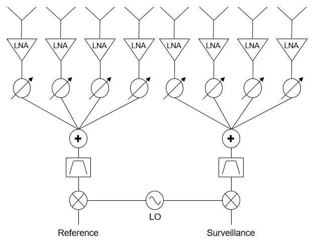
The schematic shown above represents the receiver that we will be modeling. This model will include thermal noise from the LNA, phase shift and amplitude errors from the beamformer, frequency specific effects from the filter, and phase noise from the LO.

First, we create the antenna model.

nSubElements = 4;
nDigital = 2;
nAnalog = nSubElements*nDigital;
rxULA = phased.ULA(NumElements=nAnalog,ElementSpacing=lambda/2);
rxAntenna = phased.Collector(Sensor=rxULA,OperatingFrequency=fc);

The system bandwidth is equal to the sampling rate.

bandwidth = fs;

The low noise amplifiers on the ADALM-PHASER board have a noise figure of 3.3 dB, a gain of 15.5 dB, and an OIP3 of 29 dBm.

lnaGain = 15.5;
lnaOIP3 = 29;
lnaNF = 3.3;
tEq = systemp(lnaNF);
lna = rf.Amplifier(Gain=lnaGain,OIP3=lnaOIP3,IncludeNoise=true,NoiseType="noise-temperature",NoiseTemperature=tEq,SampleRate=fs);

We use a helper class to define the analog beamformer, which applies an attenuation and phase shift on each analog channel and combines the signals. In addition to applying the requested phase shift and attenuation, this model inserts some small phase and amplitude errors to account for non-ideal behavior of real analog beamformers.

A phased.CustomCascadeComponent is used in order to insert this custom model into our receiver.

beamformer = helperPhaserBeamformer();
customBf = phased.CustomCascadeComponent(BehaviorFcn=@(x)beamformer.beamform(x),NumInputChannels=nAnalog,NumOutputChannels=nDigital,ComponentName="Beam Form");

The filter after the beamformer is a bandpass filter.

filter = rf.Filter(ResponseType='bandpass',RF=fc,PassFreq_bp=[fc-bandwidth/2 fc+bandwidth/2],SampleRate=fs);

There is a down-conversion mixer after the filter. The values used to define the mixer behavior come from the oscillator present on the ADALM-PHASER board.

fLo = 12.5e9;
fOffset = [100 10e3 100e3];
nOffset = [-80 -100 -100];
mix = rf.Mixer(Model='demod',LO=fLo,RF=fc,IncludePhaseNoise=true,SampleRate=fs,...
    PhaseNoiseFrequencyOffset=fOffset,PhaseNoiseLevel=nOffset,...
    PhaseNoiseAutoResolution=false,PhaseNoiseNumSamples=2^10);

We create the model of the receiver by cascading the individual components created above.

rx = phased.Receiver(Configuration="Cascade",Cascade={lna,customBf,filter,mix});
viewLayout(rx);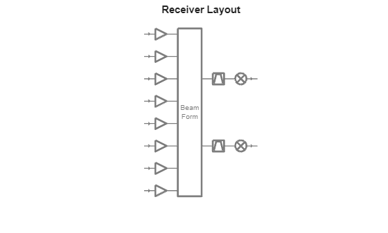

This receiver model matches the high-level schematic of the ADALM-PHASER.

Passive Radar Waveform Level Simulation

With the scenario set, and the transmitter and receiver models created, we can simulate I/Q level passive radar data. One goal of this example is to demonstrate that the final SINR measured in our simulated data resembles the measured SINR from our real-world data to validate our simulation.

One difficulty with this analysis is that there are many parameters that may vary between our simulation and real-world data collection, such as the transmit power, the target radar cross section (RCS), the location of the transmitter and target in our reference and surveillance beam patterns, etc. It is unrealistic that all of the parameters that we use in a single simulation will match the real-world parameters of the scenario in which data was collected.

We will use a Monte Carlo approach to address this issue. We will define a range of possible values for each of these unknown parameters and run many simulations with these parameters selected randomly in each simulation.

In a later section we take this distribution of possible SINR values and validate that the value from our real-world data falls within the distribution.

Single Scenario Simulation

In this section we demonstrate how to run a single simulation step and process the I/Q data before running our Monte Carlo simulations.

Signal Processing Routine

The signal processing routine used for this passive radar is discussed prior to simulating the I/Q data collection. We do so because the beamforming must be configured prior to data collection. A schematic of the routine is shown below:

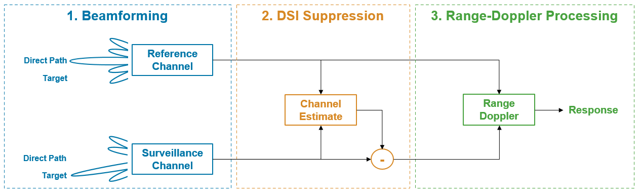
As shown above, there are three key steps used to increase the SINR to enable target detection with this passive radar system.

1. Beamforming: The reference channel antenna array is configured to focus a beam towards the transmitter to capture a clean direct path reference signal. The surveillance channel antenna array is configured to null the beam in the direction of the transmitter to reduce the impact of the direct path.

2. Direct Signal Interference (DSI) Suppression: Even with beamforming, the direct path signal power is often orders of magnitude higher than the target returns in the surveillance channel. This step removes the direct path signal from the surveillance channel. For more information on DSI suppression, see Direct Signal Interference (DSI) Suppression In Passive Radar.

3. Range-Doppler Processing: The reference channel signal is used to matched filter the surveillance channel, and the filtered signal is arranged into a cube for Doppler processing using the FFT. This can also be done by matched filtering with Doppler shifted versions of the reference channel.

This is a common approach for passive radar signal processing [1], [2]. The beamformers on the receiver model must be configured prior to simulating propagation. This is discussed in the next section.

Beamforming Setup

The analog beamformer must be configured to get a clean copy of the direct path signal in the reference channel, and to limit the impact of DSI in the surveillance channel. To do so, a null is inserted into the surveillance channel pattern in the direction of the transmitter, and the reference channel is steered in the direction of the transmitter.

The location of the transmitter can be estimated but will not be precisely known, and the location of the target can be assumed to fall somewhere on the main beam of the surveillance channel.

To demonstrate a single simulation frame, we beamform assuming that the transmitter location is known exactly, and the main beam is steered directly towards the target. In our Monte Carlo simulation, these values will be parameterized. The following steps show how the beam pattern is synthesized in the signal simulation by setting steering weights on the beamformer.

First, we get the transmitter, receiver, and target positions from the scenario and calculate the angle of the transmitter and target relative to the receiver.

% Get platform positions from scene
platforms = scene.platformPoses();
txPose = platforms(1);
rxPose = platforms(2);
targetPose = platforms(3);
clutterPose = platforms(4:end);

% Get transmit angle and target angle
[~,txAngle] = rangeangle(txPose.Position',rxPose.Position',rotmat(rxPose.Orientation,"point"));
[~,targetAngle] = rangeangle(targetPose.Position',rxPose.Position',rotmat(rxPose.Orientation,"point"));

The first channel is the reference channel, and the second channel is the surveillance channel.

refChannel = 1;
survChannel = 2;

Get the element positions for the reference and surveillance channel elements.

% Full array element position
elPos = getElementPosition(rxULA)/lambda;

% Reference channel element positions
refElStart = (refChannel-1)*nSubElements+1;
refElStop = refElStart+nSubElements-1;
refElPos = elPos(:,refElStart:refElStop);

% Surveillance channel element positions
survElStart = (survChannel-1)*nSubElements+1;
survElStop = survElStart+nSubElements-1;
survElPos = elPos(:,survElStart:survElStop);

Next, get the reference channel and surveillance channel weights using the known position of the target and the transmitter.

refWeights = steervec(refElPos,txAngle);
survWeights = nullweights(survElPos,targetAngle,txAngle);

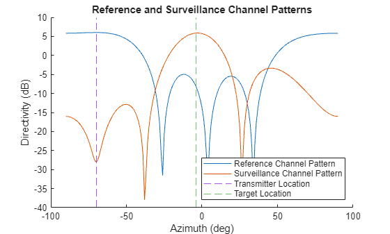
Finally, we set the steering weights on our beamformer model and plot the resultant antenna patterns.

% Apply the weights to the beamformer
beamformer.Weights = [refWeights survWeights];

% Plot the antenna pattern for the reference and surveillance channel
helperPlotBothPatterns(rxULA,fc,beamformer,txAngle,targetAngle);

Data Collection

With beamformer configured to properly steer the reference and surveillance channel, we can simulate the waveform propagation.

Create the bistaticTransmitter and bistaticReceiver objects using the transmitter, receiver, and antenna models defined above.

bistaticTx = bistaticTransmitter(Waveform=waveform,Transmitter=tx,TransmitAntenna=txAntenna);
bistaticRx = bistaticReceiver(ReceiveAntenna=rxAntenna,Receiver=rx,SampleRate=fs);

Set the RCS on the target vehicle and clutter vehicles.

% Assume RCS of 50 for target vehicle and clutter vehicles
rcs = 50;

% Set signature on target vehicle
targetPose.Signatures = rcsSignature(Pattern=pow2db(rcs));

% Set signature on clutter vehicles
nclutter = length(clutterPose);
for iClutter = 1:nclutter
    clutterPose(iClutter).Signatures = rcsSignature(Pattern=pow2db(rcs));
end

Create the propagation paths using the bistaticFreeSpacePath function.

proppaths = bistaticFreeSpacePath(fc,txPose,rxPose,[targetPose;clutterPose]);

Finally, with the radar models created and the propagation paths calculated, we generate I/Q data for the scenario of interest.

% Set receiver to capture full set of samples
bistaticRx.WindowDuration = nSamples/fs;

% Get the transmit signal
[txSig,txInfo] = transmit(bistaticTx,proppaths,0);
    
% Get the receive signal
receive(bistaticRx,txSig,txInfo,proppaths);
txInfo.StartTime = bistaticRx.WindowDuration;
iq = receive(bistaticRx,txSig,txInfo,proppaths);

Data Analysis

The data analysis for this passive radar consists of the steps described above. First, we suppress the DSI in the surveillance channel, and then we perform range-Doppler processing using the reference channel as a matched filter.

The I/Q data is separated into the reference and surveillance channel data for further processing.

ref = iq(:,refChannel);
surv = iq(:,survChannel);

For DSI suppression, we use the standard Wiener-Hopf filter.

nTaps = 100;
survClean = helperWeinerHopfFilter(ref,surv,nTaps);

We can compare the magnitude of the original surveillance data to the magnitude of the surveillance data after DSI removal.

nPlotsamples = 1000;
ax = axes(figure);
hold(ax,"on");
plot(ax,abs(surv(1:nPlotsamples)),DisplayName="Original");
plot(ax,abs(survClean(1:nPlotsamples)),DisplayName="After DSI Suppression");
title(ax,"Surveillance Channel Signal With DSI Suppression");
xlabel(ax,"Sample");
ylabel(ax,"Signal Magnitude");
legend(ax,Location="northeast");

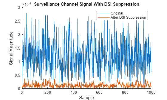
The surveillance data after DSI removal is significantly lower power because the high-power direct path and clutter returns have been suppressed.

Finally, we perform range-Doppler processing using the reference channel as the matched filter.

[resp,range,speed] = helperBistaticRangeDoppler(survClean,ref,fs,fc,200,40);

We plot the response.

helperPlotRangeDoppler(abs(resp),range,speed);

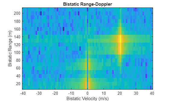
The target is clearly visible around 20 m/s velocity and 130 m range.

The last piece of the data analysis is measuring the signal-to-interference-plus-noise ratio (SINR) for our target. We do so by looking at the relative power in the range-Doppler cells where the target is known to be located, and comparing the power to an unoccupied region of the range-Doppler map which contains only noise and interference.

noiseRange = [60 200];
noiseSpeed = [-30 -10];
dirpath = proppaths(1);
tgtpath = proppaths(2);
bistaticRange = tgtpath.PathLength-dirpath.PathLength;
bistaticVel = dop2speed(tgtpath.DopplerShift,freq2wavelen(fc));
sinr = helperBistaticSINR(resp,range,speed,bistaticRange,-bistaticVel,noiseRange,noiseSpeed);
disp(['Measured SINR is ',num2str(sinr),' dB']);

Measured SINR is 39.4411 dB

The SINR is the final metric that we will measure in Monte Carlo simulations.

Monte Carlo Simulation

In this section, we measure the SINR from many simulations using the approach described in the preceding section.

Our goal in this section is to generate a distribution of SINR values that we may expect to see in our real-world data depending on the operating conditions of the system at the time of data collection.

We make many assumptions about the real system and the environment in our simulation that will not perfectly represent the real system at the time of data collection. For each of these assumptions, although we do not know a precise value, we can reasonably estimate an upper and lower bound on the true values.

Before running our simulations, we go through some of our core assumptions that we are uncertain of and assign an upper and lower bound of possible values.

The transmit power is normally a value that would be well established. The nominal output power of the amplifier being used was 100 mW. However, when measuring the power output of the amplifier used for data collection, the output power seemed to be lower than expected. We assume that the true power was between 10 and 100 mW.

pTransmitRange = [10e-3 100e-3];

The RCS of the target vehicle and other vehicles in the parking lot can vary based on many factors, including make and model, angle of incidence, angle of scattering, and operating frequency [3]. The target vehicle was a sedan; the RCS likely falls within 10 to 100 square meters.

targetRcsRange = [10 100];

The parked clutter vehicles' RCS values are assumed to take on a wider range between 10 and 300 square meters.

clutterRcsRange = [10 300];

The transmitter angle was estimated through a beam-scan approach prior to doing any bistatic radar processing. This measurement should be relatively accurate, but small errors can result in large differences in SINR because the null in the antenna pattern that suppresses the direct path signal is sharp. We assume that the estimated transmitter location is within 5 degrees of the true location.

txAngleError = [-5 5];

The target angle is unknown when doing any passive radar processing. When collecting data, we steer the beam so that the main lobe is pointing towards our surveillance area of interest. The target may fall anywhere within this surveillance area, which is assumed to be ~60 degrees wide.

rxAngleOffBoresight = [-30 30];

With these variables defined, we run the Monte Carlo simulation. In each simulation, we draw a value randomly from the uniform distribution between the upper and lower bounds that are defined.

nSims = 30;
simulatedSINR = helperRunMonteCarloSimulation(nSims,scene,bistaticTx,bistaticRx,beamformer,...
    pTransmitRange,targetRcsRange,clutterRcsRange,txAngleError,rxAngleOffBoresight,...
    noiseRange,noiseSpeed);

The following box plot shows the distribution of SINR values that were collected during simulation.

ax = axes(figure);
histogram(ax,simulatedSINR,5);
title(ax,'Distribution of Simulated SINR Values');
xlabel(ax,'SINR (dB)');

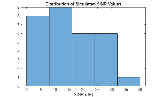
This distribution is used in the final part of the example to see if data that we collected on the real system matches our expectations from simulation.

Real World Data Collection

The setup that was used to collect data is shown in the image below. The simulated scenario in the previous section was configured to match this data collection setup.

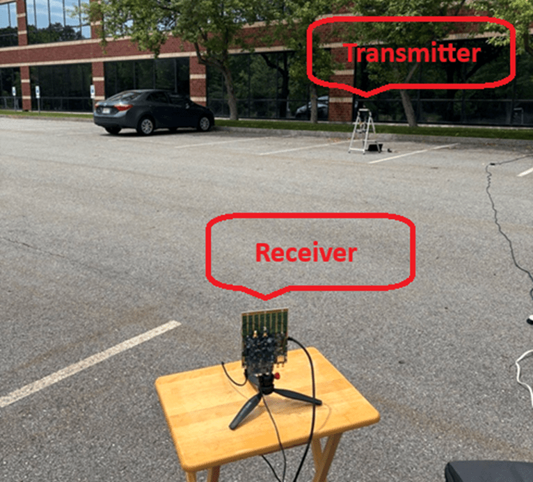
We set up one platform to act as a transmitter which is continuously transmitting a random data stream. We set up another platform to act as a receiver, and set the analog beamforming weights to steer the reference channel towards the transmitter and insert a null in the surveillance channel towards the transmitter.

A vehicle is driven through the parking lot at ~5-10 m/s. The motion is approximately radial with respect to both the transmit and receive platform, so we expect the observed Doppler frequency to correspond to a target moving at ~10-20 m/s.

The animation in the introduction shows the camera recording alongside the generated range-Doppler response from the entire data collection period. The data processing routine that was used to generate the range-Doppler response was taken directly from the previous section.

For this example, we analyze only a single data frame, which is loaded and processed below.

% Load collected data frame
load("realData.mat","rxData");
ref = rxData(:,refChannel);
surv = rxData(:,survChannel);

% Wiener filter
survClean = helperWeinerHopfFilter(ref,surv,100);

% Calculate range-Doppler Response before DSI suppression
[resp,range,speed] = helperBistaticRangeDoppler(survClean,ref,fs,fc,200,40);

% Plot range-Doppler
helperPlotRangeDoppler(abs(resp),range,speed);

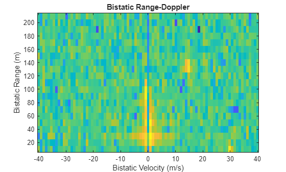
In the range-Doppler plot, a target is visible at ~15 m/s Doppler velocity and 130 m of range. The SINR is calculated using the method described in the simulation section.

% Calculate the bistatic SINR from collected data
bistaticRange = 130;
bistaticVel = 15;
measuredSinr = helperBistaticSINR(resp,range,speed,bistaticRange,bistaticVel,noiseRange,noiseSpeed);

We plot the measured SINR against the distribution of simulated SINR values.

ax = axes(figure);
histogram(ax,simulatedSINR,5,DisplayName="Simulated SINR");
title(ax,'Distribution of Simulated SINR Values');
xline(ax,measuredSinr,LineWidth=2,DisplayName="Measured SINR",LineStyle="--");
xlabel(ax,'SINR (dB)');
legend(ax);

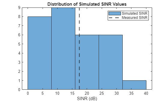
Our measured SINR falls near the mean of the simulated distribution. This validates that the simulation is a good representation of the real-world.

Conclusion

In this example, we demonstrate how to simulate and process passive radar data using a realistic system model of the ADALM-PHASER, including the effects of hardware impairments and environmental uncertainties. By following the workflow, readers learn not only how to generate and analyze simulated I/Q data, but also how to process real-world measurements using the same signal processing techniques.

A central aspect of this example is the validation of the simulation setup by direct comparison with real world data. By measuring the SINR in both simulation and the real world, we show that the simulation accurately reflects the performance observed in practice. The close agreement between simulated and measured SINR builds confidence that the simulation captures the critical aspects of the real system and environment.

This approach—systematically comparing simulation results to real world measurements—enables us to trust our simulation models for further signal processing development. With a validated simulation environment, future algorithm development, parameter tuning, and scenario exploration can be performed with greater confidence, ultimately accelerating the design and deployment of robust passive radar systems.

References

1. Garry, Joseph Landon, Chris J. Baker, and Graeme E. Smith. "Evaluation of direct signal suppression for passive radar." IEEE Transactions on Geoscience and Remote Sensing 55, no. 7 (2017): 3786-3799.

2. Palmer, James E., and Stephen J. Searle. "Evaluation of adaptive filter algorithms for clutter cancellation in passive bistatic radar." In 2012 IEEE Radar conference, pp. 0493-0498. IEEE, 2012.

3. "Vehicle Reflection". Police Radar Information Center. https://copradar.com/chapts/chapt3/ch3d6.html.

function [resp,range,speed] = helperBistaticRangeDoppler(surv,ref,fs,fc,maxRange,maxSpeed)
    % Rearrange data into columns
    ns = length(surv);
    prf = ceil(2*speed2dop(maxSpeed,freq2wavelen(fc)));
    nSamplePerPulse = ceil(fs/prf);
    nCol = floor(ns/nSamplePerPulse);
    if mod(nCol,2) == 0
        % use odd column number
        nCol = nCol - 1;
    end
    ns = nCol*nSamplePerPulse;
    surv = surv(1:ns);
    ref = ref(1:ns);
    survMat = reshape(surv,[nSamplePerPulse nCol]);
    refMat = reshape(ref,[nSamplePerPulse nCol]);

    % Get the Doppler freq shifts and speeds
    prf = 1/(nSamplePerPulse/fs);
    dopFreqs = -prf/2:prf/(nCol-1):prf/2;
    speed = dop2speed(dopFreqs,freq2wavelen(fc));

    % Get the bistatic ranges
    rangeRes = physconst('LightSpeed')/fs;
    nLag = ceil(maxRange/rangeRes);
    range = (-nLag:nLag)*rangeRes;

    % Cross correlate each surveillance with reference
    resp = zeros(length(range),nCol);
    for iCol = 1:nCol
        resp(:,iCol) = xcorr(survMat(:,iCol),refMat(:,iCol),nLag);
    end

    % FFT slow time for Doppler shift
    resp = abs(fftshift(fft(resp,[],2),2));
end

function sinr = helperBistaticSINR(resp,range,speed,bistaticRange,bistaticVel,noiseRange,noiseSpeed)
    % Get target response.
    rIdx = getTargetCells(range,bistaticRange);
    vIdx = getTargetCells(speed,bistaticVel);
    tResp = resp(rIdx,vIdx);
    tRespMag = rms(tResp,"all");

    % Get average noise response
    [~,rNoiseLowIdx] = min(abs(range-noiseRange(1)));
    [~,rNoiseUpIdx] = min(abs(range-noiseRange(2)));
    [~,vNoiseLowIdx] = min(abs(speed-noiseSpeed(1)));
    [~,vNoiseUpIdx] = min(abs(speed-noiseSpeed(2)));
    nResp = resp(rNoiseLowIdx:rNoiseUpIdx,vNoiseLowIdx:vNoiseUpIdx);
    nRespMag = rms(nResp,"all");

    sinr = mag2db(tRespMag/nRespMag);

    function cidx = getTargetCells(vec,val)
        % If there is a cell which corresponds exactly to the bistatic
        % range and velocity, select that single cell, otherwise select the
        % cells above and below. Vec must be assorted in ascending order.
        nidx = length(vec);
        vdiff = vec-val;
        equalCells = find(vdiff == 0);
        greaterCells = find(vdiff > 0);
        firstGreater = greaterCells(1);
        lesserCells = find(vdiff < 0);
        lastLesser = lesserCells(end);
        if ~isempty(equalCells)
            cidx = equalCells(1);
        elseif firstGreater == 1
            cidx = 1;
        elseif lastLesser == nidx
            cidx = nidx;
        else
            cidx = [lastLesser firstGreater];
        end
    end
end

function helperPlotRangeDoppler(resp,range,speed)
    ax = axes(figure);
    respDb = mag2db(resp);
    keepRange = range > 0;
    range = range(keepRange>0);
    respDb = respDb(keepRange,:);
    imagesc(ax,speed,range,respDb);
    ax.YDir = "Normal";
    title(ax,'Bistatic Range-Doppler');
    xlabel(ax,'Bistatic Velocity (m/s)');
    ylabel(ax,'Bistatic Range (m)');
end

function helperAddClutterTargets(scene,allx,ally)
    % Add clutter targets to the scene. Include some small velocity
    % component to model the Doppler spread of the clutter.
    for x = allx
        for y = ally
            traj = kinematicTrajectory(Position=[x y 0],Velocity=(0.01*(rand(3,1)-0.5))');
            platform(scene,Trajectory=traj);
        end
    end
end

function [scanAngles,patref,patsurv] = helperPlotBothPatterns(array,fc,bf,txAng,tarAng)
    % Capture patterns
    scanAngles = -90:90;
    patref = pattern(array,fc,scanAngles,0,Weights=[bf.AppliedWeights(:,1);zeros(size(bf.AppliedWeights(:,2)))]);
    patsurv = pattern(array,fc,scanAngles,0,Weights=[zeros(size(bf.AppliedWeights(:,1)));bf.AppliedWeights(:,2)]);

    % Create axes
    ax = axes(figure);
    hold(ax,"on");

    % Plot patterns
    plot(ax,scanAngles,patref,DisplayName='Reference Channel Pattern');
    plot(ax,scanAngles,patsurv,DisplayName='Surveillance Channel Pattern');

    % Plot transmitter and target locations
    colors = ax.ColorOrder;
    numColors = size(colors,1);
    txColor = colors(mod(3,numColors)+1, :);
    tarColor = colors(mod(4,numColors)+1, :);
    xline(ax,txAng(1),DisplayName='Transmitter Location',LineStyle='--',Color=txColor);
    xline(ax,tarAng(1),DisplayName='Target Location',LineStyle='--',Color=tarColor);

    % Update labels
    title(ax,'Reference and Surveillance Channel Patterns');
    ylabel(ax,'Directivity (dB)');
    xlabel(ax,'Azimuth (deg)');
    legend(ax,Location="southeast");
end

function survest = helperWeinerHopfFilter(ref,surv,M)
    % Compute auto-correlation and cross-correlation with conjugates
    rxx = xcorr(ref, M-1, 'biased');
    rsx = xcorr(surv, ref, M-1, 'biased');
    
    % Extract centered values (zero lag at index M)
    Rxx = toeplitz(rxx(M:end));
    rsx_vec = conj(rsx(M:end));
    
    % Solve Wiener-Hopf equation
    h = conj(Rxx \ rsx_vec);
    
    % Remove the filtered reference from surveillance
    survest = surv - filter(h,1,ref);
end

function scene = helperSetupScene()
    % Create the scene
    scene = radarScenario();

    % Rx is at the origin, with a rotation to align elements along x axis
    rxPos = [0;0;0];
    rxOrient = rotz(-90);

    % Get transmitter first in the receiver frame as that is how azimuth is
    % defined, and transform to global frame
    txDistance = 10;
    txAzimuth = -70;
    [xTx,yTx,zTx] = sph2cart(deg2rad(txAzimuth),0,txDistance);
    txPosRxFrame = [xTx;yTx;zTx];
    txPos = transpose(rxOrient)*txPosRxFrame;

    % The target position is between the x position of the transmitter and
    % receiver, at 50 m (~100 m bistatic range).
    tarX = (txPos(1)+rxPos(1))/2;
    tarY = 70;
    tarPos = [tarX;tarY;0];
    tarVel = [0;10;0];

    % Setup some information about the parking lot and parked cars
    lotWidth = 14;
    carLength = 4;
    carWidth = 2;
    carSpacing = 1;
    carDistance = tarY + 10;
    carX = [-(lotWidth+carLength)/2 (lotWidth+carLength)/2];
    carY = 0:(carWidth+carSpacing):carDistance;

    % Setup scenario - add transmitter, receiver and target
    platform(scene,Position=txPos);          
    platform(scene,Position=rxPos,Orientation=quaternion(rxOrient,"rotmat","frame"));       
    traj = kinematicTrajectory(Position=tarPos,Velocity=tarVel);
    platform(scene,Trajectory=traj);
    
    % Add parked cars - center around tx and rx
    xCenter = (rxPos(1)+txPos(1))/2;
    helperAddClutterTargets(scene,carX+xCenter,carY);

    % Plot the scene
    ax = axes(figure);
    tp = theaterPlot(Parent=ax);
    txPltr = platformPlotter(tp,Marker="^",DisplayName="TX");
    rxPltr = platformPlotter(tp,Marker="v",DisplayName="RX");
    tgtPltr = platformPlotter(tp,Marker="*",DisplayName="Target Vehicle");
    clutPltr = platformPlotter(tp,Marker="square",DisplayName="Clutter Vehicles");
    poses = platformPoses(scene);
    plotPlatform(txPltr,poses(1).Position);
    plotPlatform(rxPltr,poses(2).Position);
    plotPlatform(tgtPltr,poses(3).Position,poses(3).Velocity*0.3);
    plotPlatform(clutPltr,vertcat(poses(4:end).Position));

    % Expand the limits
    yspan = ax.YLim(2)-ax.YLim(1);
    yadjust = yspan*0.1;
    ax.YLim = [ax.YLim(1)-yadjust/2 ax.YLim(2)+yadjust/2];
    xspan = ax.XLim(2)-ax.XLim(1);
    xadjust = xspan*0.3;
    ax.XLim = [ax.XLim(1)-xadjust/2 ax.XLim(2)+xadjust/2];

    % Update the ticks
    ax.YTick = [ax.YTick(1) ax.YTick(end)];
    ax.XTick = [ax.XTick(1) ax.XTick(end)];

    % Change view to birds eye
    view(ax,[0 90]);
end

function simulatedSINR = helperRunMonteCarloSimulation(nSims,scene,bistaticTx,bistaticRx,beamformer,pTransmitRange,targetRcsRange,clutterRcsRange,txAngleErrorRange,rxAngleOffBoresightRange,noiseRange,noiseSpeed)
    % This helper function re-runs the I/Q data collection presented in the
    % main body of this example, randomly generating new parameters for
    % each simulation. The resultant SINR is measured and output for
    % further analysis.
    simulatedSINR = zeros(nSims,1);
    for iSim = 1:nSims
        % Reset the scene
        release(bistaticTx);
        release(bistaticRx);
        restart(scene);

        % Set receiver to capture full set of samples
        fs = bistaticTx.Waveform.SampleRate;
        fc = bistaticRx.ReceiveAntenna.OperatingFrequency;
        nSamples = length(bistaticTx.Waveform.CustomCode);
        bistaticRx.WindowDuration = nSamples/fs;

        % Set the transmit power
        pTransmit = helperSampleUniform(pTransmitRange);
        bistaticTx.Transmitter.PeakPower = pTransmit;

        % Get platform positions from scene
        platforms = scene.platformPoses();
        txPose = platforms(1);
        rxPose = platforms(2);
        targetPose = platforms(3);
        clutterPose = platforms(4:end);

        % Get transmit angle and target angle
        [~,txAngle] = rangeangle(txPose.Position',rxPose.Position',rotmat(rxPose.Orientation,"point"));
        [~,targetAngle] = rangeangle(targetPose.Position',rxPose.Position',rotmat(rxPose.Orientation,"point"));

        % Get the estimated transmit angle
        txAngleError = helperSampleUniform(txAngleErrorRange);
        estTxAngle = txAngle-[txAngleError;0];

        % Get the steering angle
        rxAngleOffBoresight = helperSampleUniform(rxAngleOffBoresightRange);
        steerAngle = targetAngle-[rxAngleOffBoresight;0];

        % Set the reference and surveillance channels
        refChannel = 1;
        survChannel = 2;
        nSubElements = size(beamformer.Weights,1);

        % Full array element position
        lambda = freq2wavelen(fc);
        elPos = getElementPosition(bistaticRx.ReceiveAntenna.Sensor)/lambda;        

        % Get the reference element positions
        refElStart = (refChannel-1)*nSubElements+1;
        refElStop = refElStart+nSubElements-1;
        refElPos = elPos(:,refElStart:refElStop);

        % Get the surveillance element positions
        survElStart = (survChannel-1)*nSubElements+1;
        survElStop = survElStart+nSubElements-1;
        survElPos = elPos(:,survElStart:survElStop);

        % Set the beamformer weights
        refWeights = steervec(refElPos,estTxAngle);
        survWeights = nullweights(survElPos,steerAngle,estTxAngle);
        beamformer.Weights = [refWeights survWeights];

        % Assume RCS of 50 for target vehicle and clutter vehicles
        targetRcs = helperSampleUniform(targetRcsRange);

        % Set signature on target vehicle
        targetPose.Signatures = rcsSignature(Pattern=pow2db(targetRcs));

        % Set signature on clutter vehicles
        nclutter = length(clutterPose);
        for iClutter = 1:nclutter
            clutterRcs = helperSampleUniform(clutterRcsRange);
            clutterPose(iClutter).Signatures = rcsSignature(Pattern=pow2db(clutterRcs));
        end

        % Generate propagation paths
        proppaths = bistaticFreeSpacePath(fc,txPose,rxPose,[targetPose;clutterPose]);

        % Set receiver to capture full set of samples
        bistaticRx.WindowDuration = nSamples/fs;

        % Get the transmit signal
        [txSig,txInfo] = transmit(bistaticTx,proppaths,0);

        % Get the receive signal
        receive(bistaticRx,txSig,txInfo,proppaths);
        txInfo.StartTime = bistaticRx.WindowDuration;
        iq = receive(bistaticRx,txSig,txInfo,proppaths);

        % Split the reference and surveillance channels.
        ref = iq(:,refChannel);
        surv = iq(:,survChannel);

        % DSI suppression
        nTaps = 100;
        survClean = helperWeinerHopfFilter(ref,surv,nTaps);

        % Range-Doppler Processing
        [resp,range,speed] = helperBistaticRangeDoppler(survClean,ref,fs,fc,200,40);

        % Get the bistatic range and velocity of the target
        dirpath = proppaths(1);
        tgtpath = proppaths(2);
        bistaticRange = tgtpath.PathLength-dirpath.PathLength;
        bistaticVel = dop2speed(tgtpath.DopplerShift,freq2wavelen(fc));
        simulatedSINR(iSim) = helperBistaticSINR(resp,range,speed,bistaticRange,-bistaticVel,noiseRange,noiseSpeed);
    end
end

function val = helperSampleUniform(limits)
    lower = limits(1);
    upper = limits(2);
    range = upper-lower;
    val = rand*range+lower;
end