Understanding How the Partitioning Solver Works
Learn how the Partitioning Solver works with the Nonlinear Electromechanical Circuit with Partitioning Solver example. The solver creates partitions of the model and selects the best solver for the given partition. You can use the Statistics Viewer tool to analyze how the Partitioning Solver partitions the model. The tool gives details about the each partition including the solver type and equation type.
Open the example model:
openExample('simscape/NonlinearElectromechanicalCircuitWithPartitioningSolverExample')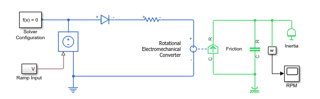
To view model statistics, in the model window, on the Debug tab, click Simscape > Statistics Viewer. Click the Update Model button to populate the viewer with data.
Select Partitions under 1-D Physical System. The solver divides the system into three partitions. One partition uses the Forward Euler solver, and the other two use Backward Euler.
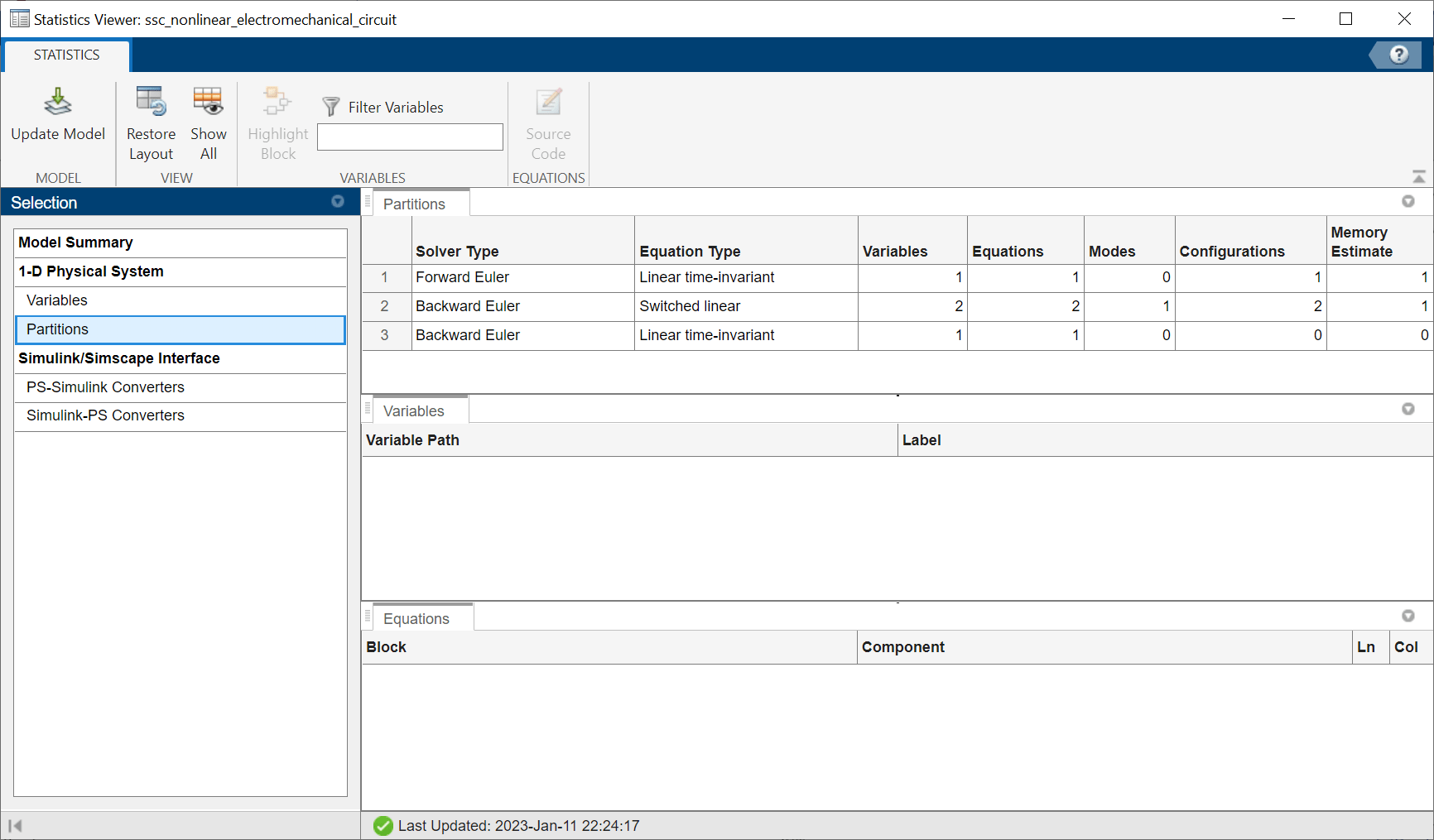
To view additional details for a partition, select the row for that partition. The Variables tab shows the variable path and label for each variable in the partition. The Equations tab shows the block and component for the partition.
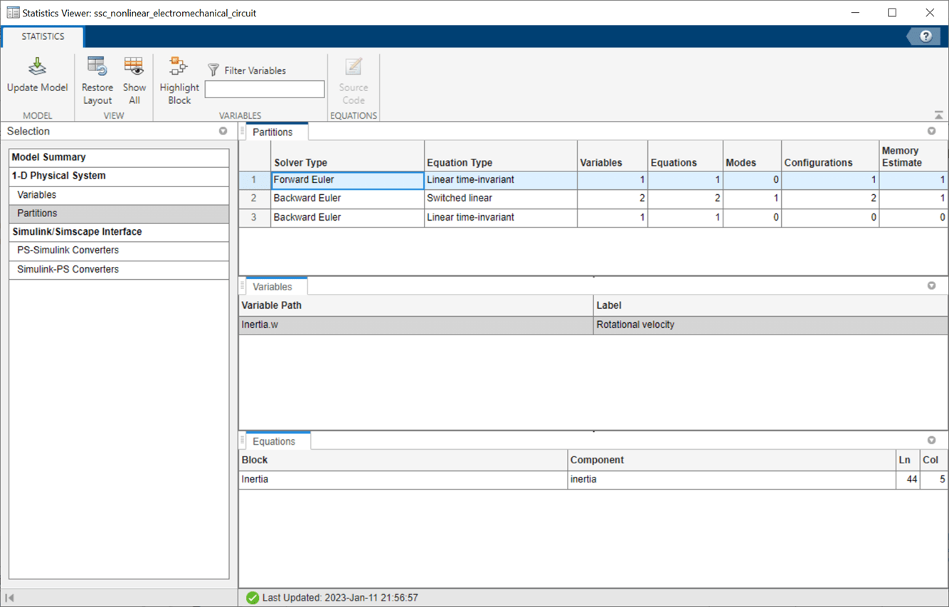
To navigate to a block in the partition, select the row for that block under either the Variables or Equations tab, and click the Highlight Block button. You can also navigate to the source code, where available, that generates a certain equation.
Select
Inertia.wunder the Variables tab, and click Source Code.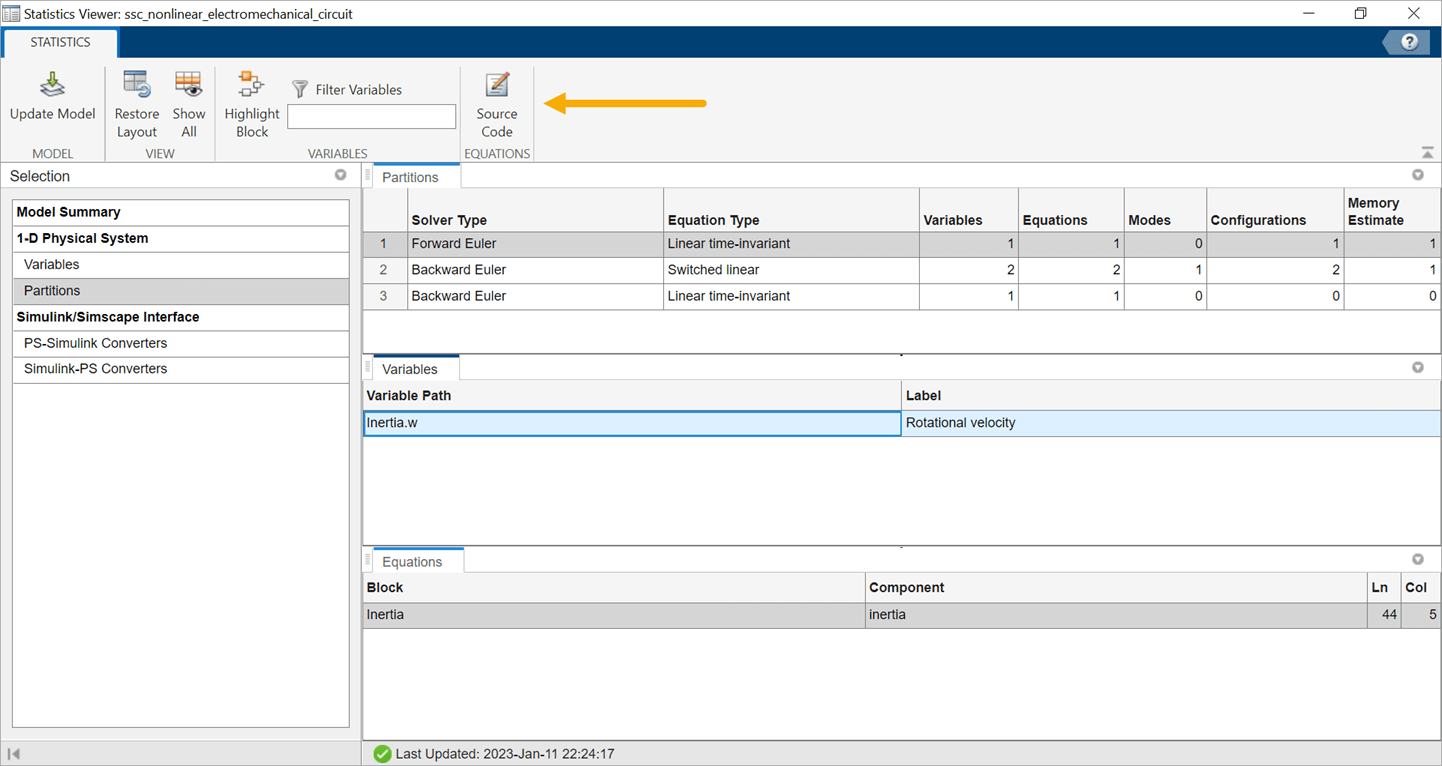
t == inertia * der(w);
Similarly, you can see the equations for other partitions.
The Partitioning Solver assembles all these equations into the system of equations required to simulate the model:
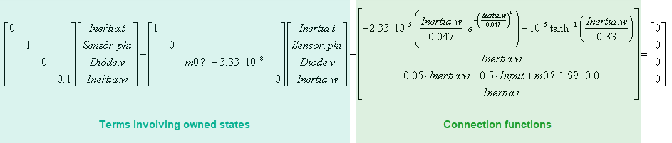
Here, Sensor.phi is the abbreviation of the Sensing.Ideal
Rotational Motion Sensor.phi variable. m0 is the boolean
originating from the equation in the Diode block, where
Diode.v is compared with the Forward voltage
parameter:
    if v > Vf
      i == (v - Vf*(1-Ron*Goff))/Ron;
    else
      i == v*Goff;
    end
Comparing this system of equations with the Statistics Viewer tool data, you
can see that the first row of the system is in Partition 3, because Partition 3 owns the
Inertia.t state variable. Similarly, the second and third rows are in
Partition 2, and the fourth row is in Partition 1.
The equation type of a partition depends only on the terms involving owned states and is not affected by the connection function. For example, Partition 3 lists its Equation Type as Linear time-invariant, despite having nonlinearities in the connection function term, because it is linear time-invariant with respect to its owned states.
During simulation, the Partitioning Solver solves the partitions in the order listed in the Statistics Viewer tool. The solver uses the updated state values, obtained after solving each partition, to perform state update for upstream partitions.