Analyze Gear Train Data and Extract Spectral Features Using Live Editor Tasks
This example shows how to use the Extract Spectral Features Live Editor task to analyze data from a current signal obtained from driving the gear train of a hobby-grade servo. The example also shows how to extract spectral features from the data to aid in fault detection and identification.
Live Editor tasks let you interactively iterate on parameters and settings while observing their effects on the result of your computation. The tasks automatically generate MATLAB® code that achieves the displayed results. For more information about Live Editor tasks generally, see Add Interactive Tasks to a Live Script.
In particular, this example uses the Extract Spectral Features Live Editor task. This task helps with analyzing and understanding spectral data. Using a comprehensive interface, you can add components to represent various bearings, gear meshes, or other parts of your hardware setup. As you set the physical parameters of these components, the Extract Spectral Features Live Editor task plots fault frequency bands at the charateristic frequencies of the components.
You can overlay power spectrum data on the fault band plot to associate various peaks in the data with the components' characteristic frequencies. This comparison can make fault detection and fault isolation easier, as you can easily trace changes in the power spectrum data back to the physical components causing them.
In addition to a plot of the characteristic frequencies and the power spectrum data, the task can generate spectral metrics of the data within each characteristic frequency band. The output metrics table containing the peak amplitude, peak frequency, and band power of each band aids in characterizing potential mechanical faults.
To run this example yourself, open the Extract Spectral Features Live Editor task and duplicate the settings that the example illustrates.
Hardware Overview

For this example, electrical current data was collected from a standard Futaba S3003 hobby servo, which was modified for continuous rotation. Servos convert the high speed of the internal DC motor to high torque at the output spline. To achieve this, servos consist of a DC motor, a set of nylon or metal drive gears, and the control circuit. The control circuit was removed to allow the current signal to the DC motor to be directly monitored. The tachometer signal at the output spline of the servo was collected using an infrared photointerrupter along with a 35 mm diameter, sixteen-slot wheel. The sixteen slots in the wheel were equally spaced and the IR photointerrupter was placed such that it emitted exactly sixteen pulses per rotation of the slotted wheel. The servo and photointerrupter were held in place by custom 3-D printed mounts.

The DC motor was driven at a constant 5 volts, and with four pairs of gears providing 278:1 speed reduction, the shaft speed at the spline was about 19.5 rpm. A second servo motor was shorted out and used as a load for the system. The current consumption was calculated using Ohm's law by measuring the voltage drop across a 0.5 ohm resistor. Since the change in current measurement values was too small for detection, the current signal was amplified using an AD22050 single-supply sensor interface amplifier. The amplified current signal was then filtered using a MAX7408 anti-aliasing fifth-order elliptic low-pass filter to smooth it and to eliminate noise before sending it to an Arduino® Uno through an analog-to-digital converter (ADC).

As the flow chart shows, the current signal was first amplified and filtered using the amplifier and the anti-aliasing low-pass filter, respectively. The Arduino Uno sampled the current signal through an ADC at 1.5 kHz and streamed it to the computer along with the tachometer pulses as serial data at a baud rate of 115,200 bps. A MATLAB script fetched the serial data from the Arduino Uno, pre-processed it, and wrote it to a .MAT file. The Extract Spectral Features Live Editor task was then used to extract the spectral metrics.
Servo Gear Train

The Futaba S3003 servo consists of four pairs of nylon gears as illustrated in this figure. The pinion P1 on the DC motor shaft meshes with the stepped gear G1. The pinion P2 is a molded part of the stepped gear G1 and meshes with the stepped gear G2. The pinion P3, which is a molded part of gear G2, meshes with the stepped gear G3. Pinion P4, which is molded with G3, meshes with the final gear G4, which is attached to the output spline. The stepped gear sets G1 and P2, G2 and P3, and G3 and P4 are free spinning gears that is, they are not attached to their respective shafts. The set of drive gears provides a 278:1 reduction, going from a motor speed of 5414.7 rpm to about 19.5 rpm at the output spline when the motor is driven at 5 volts. The following table outlines the tooth count and theoretical values of output speed, gear mesh frequencies, and cumulative gear reduction at each gear mesh.

Preprocess Data
The file servoData.mat contains two timetables corresponding to data from the servo. One timetable contains healthy data while the second timetable contains faulty data. Each data set contains about 11 seconds of data sampled at 1500 Hz.
Load the data.
load('servoData.mat', 'healthyData', 'faultyData')
healthyData
healthyData=16384×2 timetable
         Time         MotorCurrent    TachoPulse
    ______________    ____________    __________

    0 sec                307.62           1
    0.00066667 sec       301.27           1
    0.0013333 sec        309.08           1
    0.002 sec            315.92           1
    0.0026667 sec         304.2           1
    0.0033333 sec        311.04           1
    0.004 sec            311.52           1
    0.0046667 sec        305.18           1
    0.0053333 sec        315.43           0
    0.006 sec            310.06           0
    0.0066667 sec        305.66           0
    0.0073333 sec        310.55           0
    0.008 sec            304.69           0
    0.0086667 sec        310.55           0
    0.0093333 sec        310.06           0
    0.01 sec              299.8           0
      ⋮
faultyData
faultyData=16384×2 timetable
         Time         MotorCurrent    TachoPulse
    ______________    ____________    __________

    0 sec                313.48           0
    0.00066667 sec        304.2           0
    0.0013333 sec        303.22           0
    0.002 sec            319.34           0
    0.0026667 sec         304.2           0
    0.0033333 sec        303.22           0
    0.004 sec            319.82           0
    0.0046667 sec        303.22           0
    0.0053333 sec        306.64           0
    0.006 sec            321.29           0
    0.0066667 sec        303.71           0
    0.0073333 sec        308.11           0
    0.008 sec            319.34           0
    0.0086667 sec        301.76           0
    0.0093333 sec        309.08           0
    0.01 sec             319.34           0
      ⋮
Each timetable contains one column with the motor current and one column with the tacho pulse from the servo setup. In order to visualize the data in the Extract Spectral Features Live Editor task, compute the power spectrum of the motor current data. Consider the healthy data first.
fs = 1500;
[healthyMagnitudes, healthyFrequencies] = pspectrum(healthyData.MotorCurrent, healthyData.Time);
Use the Extract Spectral Features Live Editor task to plot the power spectrum data. In the task, specify healthyFrequencies for the frequency vector and healthyMagnitudes for the power spectrum magnitude.

Analyze Power Spectrum Peaks with Harmonic Fault Frequency Bands
The power spectrum plot of the servo's current data contains several noticeable peaks. You can associate these peaks with the rotating shafts in the servo setup. To determine the source of the various peaks, add components to the Extract Spectral Features Live Editor task.
To add a component to represent the first rotating shaft in the servo, enter a name for the component, select its type as Custom, and press Add. Use the output speeds in the table above to choose the frequency of the shaft component. The output speeds were computed based on the measured speed of the output shaft and the known gear reductions in the setup.
The frequency of the first shaft is 90.24 Hz. After setting the frequency value of the shaft component, note that the fault frequency band overlaps with one of the peaks in the power spectrum data at around 90 Hz. You can therefore associate this peak in large part with the first shaft. Adding in several more harmonics of the first shaft's fundamental frequency creates more fault frequency bands that overlap other peaks in the data. Harmonic frequency bands are centered around integer multiples of the fundamental frequency and can still be associated with the same component. Set the harmonics of the first shaft to be the vector [1 2 3 4 5 6] so that the fault bands spread over most of the frequency range. The first shaft is rotates at the highest frequency, so power spectrum peaks at higher frequencies are due to this shaft's harmonics.

To account for smaller power spectrum peaks such as those around 13 Hz or 29 Hz, add in a component for the second rotating shaft. This component is also a custom component, and its fundamental frequency is 14.56 Hz. You do not need to add as many harmonics for the second shaft since most of the higher peak frequencies are largely accounted for by harmonics of the first shaft. Set the harmonics of the second shaft to be the vector [1 2 3 4]. The first, second, and fourth harmonics of this shaft frequency align nicely with peaks in the power spectrum plot. However since the third harmonic is less prominent in the data, you do not need to include this harmonic. Change the harmonics of the second shaft to be the vector [1 2 4].

Similarly to the second shaft, add a component for the third rotating shaft. The fundamental frequency of this component is 2.91 Hz, as seen in the table. Start with the first four harmonics to determine if they align with any prominent peaks in the data. Note that the third harmonic of the third shaft matches a power spectrum spike around 8 Hz. The other harmonics are less prominent and can be removed. It might be the case that the frequency resolution of the power spectrum does not allow distinguishing lower frequencies. Set the harmonics of the third shaft component to be just the third harmonic.

Since the output speeds of the remaining shafts are also low frequencies that might not be distinguishable from the frequency resolution of the power spectrum, adding components for these shafts is not necessary to analyze the major peaks of the motor current data.
Analyze Sideband Peaks
By zooming into the plot in the task, you can see that the power spectrum data contains side peaks next to some of the major peaks. For instance, smaller side peaks around 76 Hz and 104 Hz surround the peak at 90 Hz. These peaks are likely associated with sidebands of the first shaft component. Sidebands are caused by a second related frequency source impacting the primary harmonic frequency source. With the servo setup, this observation leads to the presumption that the sidebands for each shaft are caused by the next shaft in the gear train.

Edit the first two shaft components to include their first sideband. For the first shaft, the sideband separation value should be equal to the nominal output frequency of the second shaft, 14.56 Hz.

Similarly for the second shaft the sideband separation value should be equal to the nominal frequency of the third shaft, 2.91 Hz. Zooming in again on the plot shows that many of the new sidebands overlap well with side peaks in the data. This is easier to see at low frequencies such as between 0 Hz and 120 Hz.

Extract Spectral Metrics to Detect Faults
The Extract Spectral Features Live Editor task generates various spectral metrics of the power spectrum data in fault frequency ranges. For each fault frequency band, compute the peak amplitude, peak frequency, and band power along with the total band power of all fault frequency bands.
load('dataSample1.mat')
spectralMetrics_healthyspectralMetrics_healthy=1×85 table
PeakAmplitude1 PeakFrequency1 BandPower1 PeakAmplitude2 PeakFrequency2 BandPower2 PeakAmplitude3 PeakFrequency3 BandPower3 PeakAmplitude4 PeakFrequency4 BandPower4 PeakAmplitude5 PeakFrequency5 BandPower5 PeakAmplitude6 PeakFrequency6 BandPower6 PeakAmplitude7 PeakFrequency7 BandPower7 PeakAmplitude8 PeakFrequency8 BandPower8 PeakAmplitude9 PeakFrequency9 BandPower9 PeakAmplitude10 PeakFrequency10 BandPower10 PeakAmplitude11 PeakFrequency11 BandPower11 PeakAmplitude12 PeakFrequency12 BandPower12 PeakAmplitude13 PeakFrequency13 BandPower13 PeakAmplitude14 PeakFrequency14 BandPower14 PeakAmplitude15 PeakFrequency15 BandPower15 PeakAmplitude16 PeakFrequency16 BandPower16 PeakAmplitude17 PeakFrequency17 BandPower17 PeakAmplitude18 PeakFrequency18 BandPower18 PeakAmplitude19 PeakFrequency19 BandPower19 PeakAmplitude20 PeakFrequency20 BandPower20 PeakAmplitude21 PeakFrequency21 BandPower21 PeakAmplitude22 PeakFrequency22 BandPower22 PeakAmplitude23 PeakFrequency23 BandPower23 PeakAmplitude24 PeakFrequency24 BandPower24 PeakAmplitude25 PeakFrequency25 BandPower25 PeakAmplitude26 PeakFrequency26 BandPower26 PeakAmplitude27 PeakFrequency27 BandPower27 PeakAmplitude28 PeakFrequency28 BandPower28 TotalBandPower
______________ ______________ __________ ______________ ______________ __________ ______________ ______________ __________ ______________ ______________ __________ ______________ ______________ __________ ______________ ______________ __________ ______________ ______________ __________ ______________ ______________ __________ ______________ ______________ __________ _______________ _______________ ___________ _______________ _______________ ___________ _______________ _______________ ___________ _______________ _______________ ___________ _______________ _______________ ___________ _______________ _______________ ___________ _______________ _______________ ___________ _______________ _______________ ___________ _______________ _______________ ___________ _______________ _______________ ___________ _______________ _______________ ___________ _______________ _______________ ___________ _______________ _______________ ___________ _______________ _______________ ___________ _______________ _______________ ___________ _______________ _______________ ___________ _______________ _______________ ___________ _______________ _______________ ___________ _______________ _______________ ___________ ______________
0.018807 77.106 0.044031 0.66362 90.842 2.2909 0.0077426 104.58 0.026419 0.0019168 168.13 0.0076763 0.038096 182.6 0.13879 0.0034959 192.86 0.013926 0.026784 258.24 0.11461 0.19204 270.7 0.68298 0.033746 284.07 0.12342 0.0026495 347.62 0.0099187 0.0048234 360.81 0.020787 0.0022197 375.64 0.0086089 0.018193 435.53 0.074193 0.041176 449.08 0.12665 0.018563 467.22 0.069274 0.96653 526.01 3.7305 0.91167 539.19 3.1072 0.29483 558.24 1.0806 1.0344 11.905 0.75499 4.2123 14.286 3.0377 0.076126 17.399 0.078413 0.037838 26.557 0.038039 0.75323 29.121 0.63973 0.010537 32.234 0.010979 0.0058568 55.311 0.006088 0.01419 58.425 0.011768 0.0033215 61.355 0.0034384 0.51018 8.7912 0.27612 16.528
These metrics may prove useful in detecting faults in the servo setup. Significant changes in the power spectrum data often indicate that some component are changing or failing. If there is a shift in one of the peak frequencies or if a peak amplitude drops significantly over time, then this may be a sign of failure.
To examine this scenario, compute the power spectrum data for the faulty data set.
[faultyMagnitudes, faultyFrequencies] = pspectrum(faultyData.MotorCurrent, faultyData.Time);
Plot the spectrum of faulty data in the task, and adjust the fundamental frequencies and sideband separation values of the shaft components based on the measured output speed of the servo setup.
Fs = 1500; % 1500 Hz [outputSpeed,t] = tachorpm(faultyData.TachoPulse,Fs,'PulsesPerRev',16,'FitType','linear'); meanOutputSpeed = mean(outputSpeed)/60 % convert from rpm to Hz
meanOutputSpeed = 0.3150
shaft4Speed = meanOutputSpeed * 41 / 16 % 16 pinion teeth, 41 gear teethshaft4Speed = 0.8072
shaft3Speed = shaft4Speed * 35 / 10 % 10 pinion teeth, 35 gear teethshaft3Speed = 2.8251
shaft2Speed = shaft3Speed * 50 / 10 % 10 pinion teeth, 50 gear teethshaft2Speed = 14.1254
shaft1Speed = shaft2Speed * 62 / 10 % 10 pinion teeth, 62 gear teethshaft1Speed = 87.5772
For the first shaft component, use shaft1Speed as the fundamental frequency and shaft2Speed as the sideband separation. For the second shaft component, use shaft2Speed as the fundamental frequency and shaft3Speed as the sideband separation. For the third shaft component, use shaft3Speed as the fundamental frequency.

As can be seen in the visualization of the faulty power spectrum data, several of the peaks have diminished in magnitude. For example, the peak aligned in the healthy dataset with the second harmonic of the first shaft around 180 Hz is almost negligible in the faulty dataset. Since it was previously determined that this peak is likely associated with the first shaft, this indicates a potential failure in the first shaft. Further examination of the spectral metrics table can provide more detailed information about the peak frequencies, peak amplitudes, and band powers.
spectralMetrics_faulty
spectralMetrics_faulty=1×85 table
PeakAmplitude1 PeakFrequency1 BandPower1 PeakAmplitude2 PeakFrequency2 BandPower2 PeakAmplitude3 PeakFrequency3 BandPower3 PeakAmplitude4 PeakFrequency4 BandPower4 PeakAmplitude5 PeakFrequency5 BandPower5 PeakAmplitude6 PeakFrequency6 BandPower6 PeakAmplitude7 PeakFrequency7 BandPower7 PeakAmplitude8 PeakFrequency8 BandPower8 PeakAmplitude9 PeakFrequency9 BandPower9 PeakAmplitude10 PeakFrequency10 BandPower10 PeakAmplitude11 PeakFrequency11 BandPower11 PeakAmplitude12 PeakFrequency12 BandPower12 PeakAmplitude13 PeakFrequency13 BandPower13 PeakAmplitude14 PeakFrequency14 BandPower14 PeakAmplitude15 PeakFrequency15 BandPower15 PeakAmplitude16 PeakFrequency16 BandPower16 PeakAmplitude17 PeakFrequency17 BandPower17 PeakAmplitude18 PeakFrequency18 BandPower18 PeakAmplitude19 PeakFrequency19 BandPower19 PeakAmplitude20 PeakFrequency20 BandPower20 PeakAmplitude21 PeakFrequency21 BandPower21 PeakAmplitude22 PeakFrequency22 BandPower22 PeakAmplitude23 PeakFrequency23 BandPower23 PeakAmplitude24 PeakFrequency24 BandPower24 PeakAmplitude25 PeakFrequency25 BandPower25 PeakAmplitude26 PeakFrequency26 BandPower26 PeakAmplitude27 PeakFrequency27 BandPower27 PeakAmplitude28 PeakFrequency28 BandPower28 TotalBandPower
______________ ______________ __________ ______________ ______________ __________ ______________ ______________ __________ ______________ ______________ __________ ______________ ______________ __________ ______________ ______________ __________ ______________ ______________ __________ ______________ ______________ __________ ______________ ______________ __________ _______________ _______________ ___________ _______________ _______________ ___________ _______________ _______________ ___________ _______________ _______________ ___________ _______________ _______________ ___________ _______________ _______________ ___________ _______________ _______________ ___________ _______________ _______________ ___________ _______________ _______________ ___________ _______________ _______________ ___________ _______________ _______________ ___________ _______________ _______________ ___________ _______________ _______________ ___________ _______________ _______________ ___________ _______________ _______________ ___________ _______________ _______________ ___________ _______________ _______________ ___________ _______________ _______________ ___________ _______________ _______________ ___________ ______________
0.0011027 75.641 0.003537 0.032586 88.095 0.095873 0.00095284 101.47 0.00395 0.00041757 158.97 0.0016883 0.0010558 174.73 0.0038404 0.00041803 190.11 0.0018164 0.0051769 249.27 0.017515 0.02861 261.54 0.12024 0.0050995 274.91 0.015488 0.0014899 336.08 0.0062536 0.0034166 350.37 0.0151 0.0014213 363.19 0.0049667 0.0022729 423.63 0.0092143 0.0058396 437.36 0.020548 0.0031547 450.37 0.010476 1.9385 511.36 6.3395 1.3398 523.81 5.1888 0.79239 539.38 2.9425 0.99793 11.538 0.82466 2.7276 13.919 1.9334 0.03098 17.033 0.03294 0.019366 25.641 0.018542 0.27042 28.205 0.26876 0.0056307 31.136 0.0060665 0.0029552 54.029 0.0028713 0.024583 56.593 0.025096 0.002738 58.974 0.0027415 0.74611 8.4249 0.40382 18.32
As an alternative to updating the spectral data in the Live Editor task, you can also use the automatically generated MATLAB code to determine the spectral metrics of the faulty data. The code below was automatically generated when the Live Editor task was used to generate the healthy spectral metrics. Execute the code.
% Generate the fault bands and information for each component [FB_Shaft1, info_Shaft1] = faultBands(90.24, 1:6, 14.56, 0:1); [FB_Shaft2, info_Shaft2] = faultBands(14.56, [1 2 4], 2.91, 0:1); [FB_Shaft3, info_Shaft3] = faultBands(2.91, 3); % Combine the fault bands of each component FB_healthy = [FB_Shaft1; ... FB_Shaft2; ... FB_Shaft3]; % Combine the information regarding the fault bands of each component info_healthy.Centers = [info_Shaft1.Centers, ... info_Shaft2.Centers, ... info_Shaft3.Centers]; info_healthy.Labels = [info_Shaft1.Labels, ... info_Shaft2.Labels, ... info_Shaft3.Labels]; info_healthy.FaultGroups = [info_Shaft1.HarmonicGroups, ... info_Shaft2.HarmonicGroups, ... info_Shaft3.HarmonicGroups]; % Clear temporary outputs from the workspace clear FB_Shaft1 info_Shaft1; clear FB_Shaft2 info_Shaft2; clear FB_Shaft3 info_Shaft3; % Compute fault band metrics of the power spectrum healthyMagnitudes spectralMetrics_healthy = faultBandMetrics(healthyMagnitudes, healthyFrequencies, FB_healthy)
spectralMetrics_healthy=1×85 table
    PeakAmplitude1    PeakFrequency1    BandPower1    PeakAmplitude2    PeakFrequency2    BandPower2    PeakAmplitude3    PeakFrequency3    BandPower3    PeakAmplitude4    PeakFrequency4    BandPower4    PeakAmplitude5    PeakFrequency5    BandPower5    PeakAmplitude6    PeakFrequency6    BandPower6    PeakAmplitude7    PeakFrequency7    BandPower7    PeakAmplitude8    PeakFrequency8    BandPower8    PeakAmplitude9    PeakFrequency9    BandPower9    PeakAmplitude10    PeakFrequency10    BandPower10    PeakAmplitude11    PeakFrequency11    BandPower11    PeakAmplitude12    PeakFrequency12    BandPower12    PeakAmplitude13    PeakFrequency13    BandPower13    PeakAmplitude14    PeakFrequency14    BandPower14    PeakAmplitude15    PeakFrequency15    BandPower15    PeakAmplitude16    PeakFrequency16    BandPower16    PeakAmplitude17    PeakFrequency17    BandPower17    PeakAmplitude18    PeakFrequency18    BandPower18    PeakAmplitude19    PeakFrequency19    BandPower19    PeakAmplitude20    PeakFrequency20    BandPower20    PeakAmplitude21    PeakFrequency21    BandPower21    PeakAmplitude22    PeakFrequency22    BandPower22    PeakAmplitude23    PeakFrequency23    BandPower23    PeakAmplitude24    PeakFrequency24    BandPower24    PeakAmplitude25    PeakFrequency25    BandPower25    PeakAmplitude26    PeakFrequency26    BandPower26    PeakAmplitude27    PeakFrequency27    BandPower27    PeakAmplitude28    PeakFrequency28    BandPower28    TotalBandPower
    ______________    ______________    __________    ______________    ______________    __________    ______________    ______________    __________    ______________    ______________    __________    ______________    ______________    __________    ______________    ______________    __________    ______________    ______________    __________    ______________    ______________    __________    ______________    ______________    __________    _______________    _______________    ___________    _______________    _______________    ___________    _______________    _______________    ___________    _______________    _______________    ___________    _______________    _______________    ___________    _______________    _______________    ___________    _______________    _______________    ___________    _______________    _______________    ___________    _______________    _______________    ___________    _______________    _______________    ___________    _______________    _______________    ___________    _______________    _______________    ___________    _______________    _______________    ___________    _______________    _______________    ___________    _______________    _______________    ___________    _______________    _______________    ___________    _______________    _______________    ___________    _______________    _______________    ___________    _______________    _______________    ___________    ______________

       0.018807           77.106         0.044031        0.66362            90.842          2.2909        0.0077426           104.58         0.026419       0.0019168           168.13        0.0076763        0.038096           182.6          0.13879        0.0034959           192.86         0.013926        0.026784           258.24         0.11461         0.19204            270.7          0.68298         0.033746           284.07         0.12342         0.0026495           347.62          0.0099187        0.0048234           360.81          0.020787         0.0022197           375.64          0.0086089        0.018193            435.53          0.074193         0.041176            449.08           0.12665         0.018563            467.22          0.069274          0.96653            526.01           3.7305           0.91167            539.19           3.1072           0.29483            558.24           1.0806           1.0344             11.905           0.75499          4.2123             14.286           3.0377          0.076126            17.399          0.078413         0.037838            26.557          0.038039          0.75323            29.121           0.63973         0.010537            32.234          0.010979         0.0058568           55.311          0.006088          0.01419            58.425          0.011768         0.0033215           61.355          0.0034384         0.51018            8.7912           0.27612          16.528
This code can easily be adjusted for the new faulty dataset.
% Generate the fault bands and information for each component [FB_Shaft1, info_Shaft1] = faultBands(shaft1Speed, 1:6, shaft2Speed, 0:1); [FB_Shaft2, info_Shaft2] = faultBands(shaft2Speed, [1 2 4], shaft3Speed, 0:1); [FB_Shaft3, info_Shaft3] = faultBands(shaft3Speed, 3); % Combine the fault bands of each component FB_faulty = [FB_Shaft1; ... FB_Shaft2; ... FB_Shaft3]; % Combine the information regarding the fault bands of each component info_faulty.Centers = [info_Shaft1.Centers, ... info_Shaft2.Centers, ... info_Shaft3.Centers]; info_faulty.Labels = [info_Shaft1.Labels, ... info_Shaft2.Labels, ... info_Shaft3.Labels]; info_faulty.FaultGroups = [info_Shaft1.HarmonicGroups, ... info_Shaft2.HarmonicGroups, ... info_Shaft3.HarmonicGroups]; % Clear temporary outputs from the workspace clear FB_Shaft1 info_Shaft1; clear FB_Shaft2 info_Shaft2; clear FB_Shaft3 info_Shaft3; % Compute fault band metrics of the power spectrum healthyMagnitudes spectralMetrics_faulty = faultBandMetrics(faultyMagnitudes, faultyFrequencies, FB_faulty)
spectralMetrics_faulty=1×85 table
    PeakAmplitude1    PeakFrequency1    BandPower1    PeakAmplitude2    PeakFrequency2    BandPower2    PeakAmplitude3    PeakFrequency3    BandPower3    PeakAmplitude4    PeakFrequency4    BandPower4    PeakAmplitude5    PeakFrequency5    BandPower5    PeakAmplitude6    PeakFrequency6    BandPower6    PeakAmplitude7    PeakFrequency7    BandPower7    PeakAmplitude8    PeakFrequency8    BandPower8    PeakAmplitude9    PeakFrequency9    BandPower9    PeakAmplitude10    PeakFrequency10    BandPower10    PeakAmplitude11    PeakFrequency11    BandPower11    PeakAmplitude12    PeakFrequency12    BandPower12    PeakAmplitude13    PeakFrequency13    BandPower13    PeakAmplitude14    PeakFrequency14    BandPower14    PeakAmplitude15    PeakFrequency15    BandPower15    PeakAmplitude16    PeakFrequency16    BandPower16    PeakAmplitude17    PeakFrequency17    BandPower17    PeakAmplitude18    PeakFrequency18    BandPower18    PeakAmplitude19    PeakFrequency19    BandPower19    PeakAmplitude20    PeakFrequency20    BandPower20    PeakAmplitude21    PeakFrequency21    BandPower21    PeakAmplitude22    PeakFrequency22    BandPower22    PeakAmplitude23    PeakFrequency23    BandPower23    PeakAmplitude24    PeakFrequency24    BandPower24    PeakAmplitude25    PeakFrequency25    BandPower25    PeakAmplitude26    PeakFrequency26    BandPower26    PeakAmplitude27    PeakFrequency27    BandPower27    PeakAmplitude28    PeakFrequency28    BandPower28    TotalBandPower
    ______________    ______________    __________    ______________    ______________    __________    ______________    ______________    __________    ______________    ______________    __________    ______________    ______________    __________    ______________    ______________    __________    ______________    ______________    __________    ______________    ______________    __________    ______________    ______________    __________    _______________    _______________    ___________    _______________    _______________    ___________    _______________    _______________    ___________    _______________    _______________    ___________    _______________    _______________    ___________    _______________    _______________    ___________    _______________    _______________    ___________    _______________    _______________    ___________    _______________    _______________    ___________    _______________    _______________    ___________    _______________    _______________    ___________    _______________    _______________    ___________    _______________    _______________    ___________    _______________    _______________    ___________    _______________    _______________    ___________    _______________    _______________    ___________    _______________    _______________    ___________    _______________    _______________    ___________    _______________    _______________    ___________    ______________

      0.0011027           75.641         0.003537        0.032586           88.095         0.095873       0.00095284          101.47         0.00395        0.00041757          158.97        0.0016883       0.0010558           174.73        0.0038404       0.00041803          190.11        0.0018164       0.0051769           249.27         0.017515        0.02861            261.54         0.12024        0.0050995           274.91         0.015488        0.0014899           336.08          0.0062536        0.0034166           350.37           0.0151          0.0014213           363.19          0.0049667        0.0022729           423.63          0.0092143        0.0058396           437.36          0.020548         0.0031547           450.37          0.010476          1.9385             511.36           6.3395           1.3398             523.81           5.1888           0.79239            539.38           2.9425           0.99793            11.538           0.82466          2.7276             13.919           1.9334           0.03098            17.033           0.03294         0.019366            25.641          0.018542          0.27042            28.205           0.26876         0.0056307           31.136          0.0060665        0.0029552           54.029          0.0028713        0.024583            56.593          0.025096         0.002738            58.974          0.0027415         0.74611            8.4249           0.40382          18.32
Combining the healthy and faulty spectral metrics tables improves visibility into changes in peak amplitudes and band powers of the spectral data.
spectralMetrics_total = [spectralMetrics_healthy; spectralMetrics_faulty]
spectralMetrics_total=2×85 table
    PeakAmplitude1    PeakFrequency1    BandPower1    PeakAmplitude2    PeakFrequency2    BandPower2    PeakAmplitude3    PeakFrequency3    BandPower3    PeakAmplitude4    PeakFrequency4    BandPower4    PeakAmplitude5    PeakFrequency5    BandPower5    PeakAmplitude6    PeakFrequency6    BandPower6    PeakAmplitude7    PeakFrequency7    BandPower7    PeakAmplitude8    PeakFrequency8    BandPower8    PeakAmplitude9    PeakFrequency9    BandPower9    PeakAmplitude10    PeakFrequency10    BandPower10    PeakAmplitude11    PeakFrequency11    BandPower11    PeakAmplitude12    PeakFrequency12    BandPower12    PeakAmplitude13    PeakFrequency13    BandPower13    PeakAmplitude14    PeakFrequency14    BandPower14    PeakAmplitude15    PeakFrequency15    BandPower15    PeakAmplitude16    PeakFrequency16    BandPower16    PeakAmplitude17    PeakFrequency17    BandPower17    PeakAmplitude18    PeakFrequency18    BandPower18    PeakAmplitude19    PeakFrequency19    BandPower19    PeakAmplitude20    PeakFrequency20    BandPower20    PeakAmplitude21    PeakFrequency21    BandPower21    PeakAmplitude22    PeakFrequency22    BandPower22    PeakAmplitude23    PeakFrequency23    BandPower23    PeakAmplitude24    PeakFrequency24    BandPower24    PeakAmplitude25    PeakFrequency25    BandPower25    PeakAmplitude26    PeakFrequency26    BandPower26    PeakAmplitude27    PeakFrequency27    BandPower27    PeakAmplitude28    PeakFrequency28    BandPower28    TotalBandPower
    ______________    ______________    __________    ______________    ______________    __________    ______________    ______________    __________    ______________    ______________    __________    ______________    ______________    __________    ______________    ______________    __________    ______________    ______________    __________    ______________    ______________    __________    ______________    ______________    __________    _______________    _______________    ___________    _______________    _______________    ___________    _______________    _______________    ___________    _______________    _______________    ___________    _______________    _______________    ___________    _______________    _______________    ___________    _______________    _______________    ___________    _______________    _______________    ___________    _______________    _______________    ___________    _______________    _______________    ___________    _______________    _______________    ___________    _______________    _______________    ___________    _______________    _______________    ___________    _______________    _______________    ___________    _______________    _______________    ___________    _______________    _______________    ___________    _______________    _______________    ___________    _______________    _______________    ___________    _______________    _______________    ___________    ______________

       0.018807           77.106         0.044031         0.66362           90.842           2.2909        0.0077426          104.58         0.026419        0.0019168          168.13        0.0076763        0.038096            182.6          0.13879        0.0034959          192.86         0.013926        0.026784           258.24          0.11461        0.19204             270.7         0.68298         0.033746           284.07          0.12342        0.0026495           347.62          0.0099187        0.0048234           360.81          0.020787         0.0022197           375.64          0.0086089         0.018193           435.53           0.074193         0.041176           449.08           0.12665          0.018563           467.22          0.069274          0.96653            526.01           3.7305           0.91167            539.19           3.1072           0.29483            558.24           1.0806            1.0344            11.905           0.75499          4.2123             14.286           3.0377          0.076126            17.399          0.078413         0.037838            26.557          0.038039          0.75323            29.121           0.63973          0.010537           32.234           0.010979        0.0058568           55.311           0.006088         0.01419            58.425          0.011768         0.0033215           61.355          0.0034384         0.51018            8.7912           0.27612          16.528
      0.0011027           75.641         0.003537        0.032586           88.095         0.095873       0.00095284          101.47          0.00395       0.00041757          158.97        0.0016883       0.0010558           174.73        0.0038404       0.00041803          190.11        0.0018164       0.0051769           249.27         0.017515        0.02861            261.54         0.12024        0.0050995           274.91         0.015488        0.0014899           336.08          0.0062536        0.0034166           350.37            0.0151         0.0014213           363.19          0.0049667        0.0022729           423.63          0.0092143        0.0058396           437.36          0.020548         0.0031547           450.37          0.010476           1.9385            511.36           6.3395            1.3398            523.81           5.1888           0.79239            539.38           2.9425           0.99793            11.538           0.82466          2.7276             13.919           1.9334           0.03098            17.033           0.03294         0.019366            25.641          0.018542          0.27042            28.205           0.26876         0.0056307           31.136          0.0060665        0.0029552           54.029          0.0028713        0.024583            56.593          0.025096          0.002738           58.974          0.0027415         0.74611            8.4249           0.40382           18.32
For example, if you look at PeakAmplitude2 in the table, the amplitude of the power spectrum peak drops from 2.0259 to 0.0829. Using the PeakFrequency2 value, you know that this drop occurs around 90 Hz. Plot the two power spectrums on the same axes to visualize the drop outside of the Live Editor task.
plot(healthyFrequencies,10*log10(healthyMagnitudes),'b-'); % plot in decibels
hold on;
plot(faultyFrequencies,10*log10(faultyMagnitudes),'r-'); % plot in decibels
legend('Healthy','Faulty')
xlabel('Frequency (Hz)')
ylabel('Power Spectrum (dB)')
title('Comparison of Power Spectrums')
hold off;
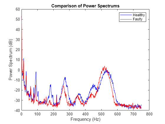
As the metrics table showed, the peak around 90 Hz drops significantly in amplitude. To determine which component frequency caused this, check back in the previous Extract Spectral Feature Live Editor task.
The fault band around 90 Hz is the first harmonic of the first rotating shaft. Thus you know that something is changing in this shaft and it may be trending towards failure.
Plotting the healthy and faulty power spectrums together can be a useful way to highlight changes in peak amplitudes. In addition to the peak around 90 Hz for the first harmonic of the first shaft, other significant decreases in peak amplitudes can be seen such as with the second harmonic of this shaft around 180 Hz. This peak is essentially nonexistent in the faulty dataset.
Peak amplitudes from the healthy and faulty data can also be compared using a bar chart.
PeakFrequencies = spectralMetrics_total(:,2:3:end-1).Variables';
PeakAmplitudes = spectralMetrics_total(:,1:3:end-1).Variables';
bar(PeakFrequencies, PeakAmplitudes);
legend('Healthy','Faulty')
xlabel('Frequency (Hz)')
ylabel('Peak Amplitude')
title('Peak Amplitudes of Healthy and Faulty Power Spectrum Data')
Zoom in to see the change in peak amplitude at the first harmonic of the first rotating shaft.
xlim([87 93])
ylim([0 0.7])

Uses of the Extract Spectral Features Live Editor Task
As shown in this example the Extract Spectral Features Live Editor task can prove useful for several different applications. With the Live Editor task, you can easily match spectral peaks with known machine component frequencies. This helps you better understand your data and the mechanical components causing various features in the data.
Another application of the Extract Spectral Features Live Editor task is to generate metrics which characterize your spectral data in the frequency ranges of interest. The task produces an output table containing the peak amplitude, peak frequency, and band power of each fault frequency band, as well as the total band power of all fault bands. However, these metrics are specific to the power spectrum data input in the task.
To extend this use so that you can track metrics over time as new data sets are gathered, you can either update the power spectrum data in the task or use the automatically generated MATLAB code to produce the metrics table. Copying the generated MATLAB code is an easy way to continue computing fault band metrics for many new data sets.
A third use of the task combines the benefits of the two previously discussed uses. Since the task associates the various mechanical components with peaks in the spectral data, you can quickly determine which components cause significant changes in the spectral data and thus potential failures. For example, one common indicator of machine failure derived from spectral data is a change in the amplitude of spectral peaks. In the spectral metrics table, if you notice a significant drop in peak amplitude or band power over time you can trace the corresponding peak frequency back to the plot to see which component's fault frequency band aligns with that peak.
See Also
faultBands | bearingFaultBands | gearMeshFaultBands | faultBandMetrics | Extract
Spectral Features