Multi-Class Fault Detection Using Simulated Data
This example shows how to use a Simulink® model to generate fault and healthy data. The data is used to develop a multi-class classifier to detect different combinations of faults. The example uses a triplex reciprocating pump model and includes leak, blocking, and bearing faults.
Set Up the Model
This example uses many supporting files that are stored in a zip file. Unzip the file to get access to the supporting files, and load the model parameters.
unzip('pdmRecipPump_supportingfiles.zip')

% Load Parameters
pdmRecipPump_Parameters %Pump
CAT_Pump_1051_DataFile_imported %CAD
Reciprocating Pump Model
The reciprocating pump consists of an electric motor, the pump housing, pump crank and pump plungers.
mdl = 'pdmRecipPump';
open_system(mdl)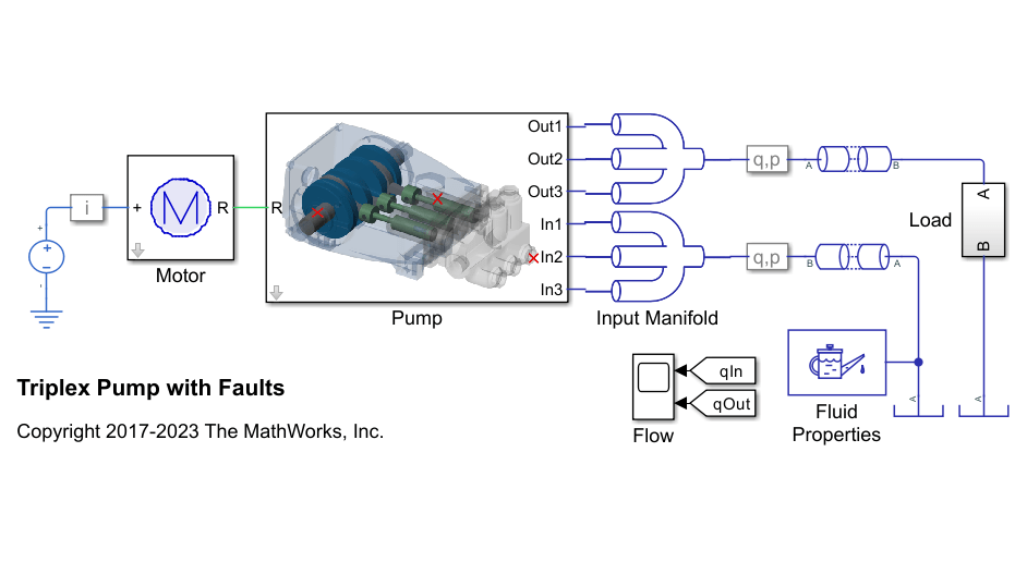
open_system([mdl,'/Pump'])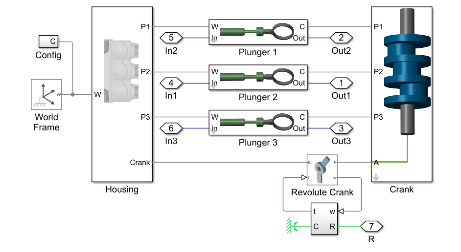
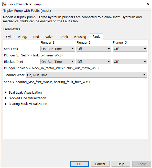
The pump model is configured to model three types of faults; cylinder leaks, blocked inlet, and increased bearing friction. These faults are parameterized as workspace variables and configured through the pump block dialog.
Simulating Fault and Healthy Data
For each of the three fault types create an array of values that represent the fault severity, ranging from no fault to a significant fault.
% Define fault parameter variations
numParValues = 10;
leak_area_set_factor = linspace(0.00,0.036,numParValues);
leak_area_set = leak_area_set_factor*TRP_Par.Check_Valve.In.Max_Area;
leak_area_set = max(leak_area_set,1e-9); % Leakage area cannot be 0
blockinfactor_set = linspace(0.8,0.53,numParValues);
bearingfactor_set = linspace(0,6e-4,numParValues);
The pump model is configured to include noise, thus running the model with the same fault parameter values will result in different simulation outputs. This is useful for developing a classifier as it means there can be multiple simulation results for the same fault condition and severity. To configure simulations for such results, create vectors of fault parameter values where the values represent no faults, a single fault, combinations of two faults, and combinations of three faults. For each group (no fault, single fault, etc.) create 125 combinations of fault values from the fault parameter values defined above. This gives a total of 1000 combinations of fault parameter values. Note that running these 1000 simulations in parallel takes around an hour on a standard desktop and generates around 620MB of data. To reduce simulation time, reduce the number of fault combinations to 20 by changing runAll = true to runAll = false. Note that a larger dataset results in a more robust classifier.
% Set number of elements in each fault group
runAll = true;
if runAll
    % Create a large dataset to build a robust classifier
    nPerGroup = 100;
else
    % Create a smaller dataset to reduce simulation time
    nPerGroup = 20; %#ok<UNRCH>
end

rng('default');    % Feed default seed to rng (Random number generator)

% No fault simulations
leakArea = repmat(leak_area_set(1),nPerGroup,1);
blockingFactor = repmat(blockinfactor_set(1),nPerGroup,1);
bearingFactor = repmat(bearingfactor_set(1),nPerGroup,1);

% Single fault simulations
idx = ceil(10*rand(nPerGroup,1));
leakArea = [leakArea; leak_area_set(idx)'];
blockingFactor = [blockingFactor;repmat(blockinfactor_set(1),nPerGroup,1)];
bearingFactor = [bearingFactor;repmat(bearingfactor_set(1),nPerGroup,1)];
idx = ceil(10*rand(nPerGroup,1));
leakArea = [leakArea; repmat(leak_area_set(1),nPerGroup,1)];
blockingFactor = [blockingFactor;blockinfactor_set(idx)'];
bearingFactor = [bearingFactor;repmat(bearingfactor_set(1),nPerGroup,1)];
idx = ceil(10*rand(nPerGroup,1));
leakArea = [leakArea; repmat(leak_area_set(1),nPerGroup,1)];
blockingFactor = [blockingFactor;repmat(blockinfactor_set(1),nPerGroup,1)];
bearingFactor = [bearingFactor;bearingfactor_set(idx)'];

% Double fault simulations
idxA = ceil(10*rand(nPerGroup,1));
idxB = ceil(10*rand(nPerGroup,1));
leakArea = [leakArea; leak_area_set(idxA)'];
blockingFactor = [blockingFactor;blockinfactor_set(idxB)'];
bearingFactor = [bearingFactor;repmat(bearingfactor_set(1),nPerGroup,1)];
idxA = ceil(10*rand(nPerGroup,1));
idxB = ceil(10*rand(nPerGroup,1));
leakArea = [leakArea; leak_area_set(idxA)'];
blockingFactor = [blockingFactor;repmat(blockinfactor_set(1),nPerGroup,1)];
bearingFactor = [bearingFactor;bearingfactor_set(idxB)'];
idxA = ceil(10*rand(nPerGroup,1));
idxB = ceil(10*rand(nPerGroup,1));
leakArea = [leakArea; repmat(leak_area_set(1),nPerGroup,1)];
blockingFactor = [blockingFactor;blockinfactor_set(idxA)'];
bearingFactor = [bearingFactor;bearingfactor_set(idxB)'];

% Triple fault simulations
idxA = ceil(10*rand(nPerGroup,1));
idxB = ceil(10*rand(nPerGroup,1));
idxC = ceil(10*rand(nPerGroup,1));
leakArea = [leakArea; leak_area_set(idxA)'];
blockingFactor = [blockingFactor;blockinfactor_set(idxB)'];
bearingFactor = [bearingFactor;bearingfactor_set(idxC)'];
Use the fault parameter combinations to create Simulink.SimulationInput objects. For each simulation input ensure that the random seed is set differently to generate different results.
for ct = numel(leakArea):-1:1
    simInput(ct) = Simulink.SimulationInput(mdl);
    simInput(ct) = setVariable(simInput(ct),'leak_cyl_area_WKSP',leakArea(ct));
    simInput(ct) = setVariable(simInput(ct),'block_in_factor_WKSP',blockingFactor(ct));
    simInput(ct) = setVariable(simInput(ct),'bearing_fault_frict_WKSP',bearingFactor(ct));
    simInput(ct) = setVariable(simInput(ct),'noise_seed_offset_WKSP',ct-1);
end
Use the generateSimulationEnsemble function to run the simulations defined by the Simulink.SimulationInput objects defined above and store the results in a local sub-folder. Then create a simulationEnsembleDatastore from the stored results.
% Run the simulation and create an ensemble to manage the simulation
% results

if isfolder('./Data')
    % Delete existing mat files
    delete('./Data/*.mat')
end

[ok,e] = generateSimulationEnsemble(simInput,fullfile('.','Data'),'UseParallel',false,'ShowProgress',false);    %Set the UseParallel flag to true to use parallel computing capabilities
ens = simulationEnsembleDatastore(fullfile('.','Data'));
Processing and Extracting Features from the Simulation Results
The model is configured to log the pump output pressure, output flow, motor speed and motor current.
ens.DataVariables
ans = 8×1 string array
    "SimulationInput"
    "SimulationMetadata"
    "iMotor_meas"
    "pIn_meas"
    "pOut_meas"
    "qIn_meas"
    "qOut_meas"
    "wMotor_meas"
For each member in the ensemble preprocess the pump output flow and compute condition indicators based on the pump output flow. The condition indicators are later used for fault classification. For preprocessing remove the first 0.8 seconds of the output flow as this contains transients from simulation and pump startup. As part of the preprocessing compute the power spectrum of the output flow, and use the SimulationInput to return the values of the fault variables.
Configure the ensemble so that the read only returns the variables of interest and call the preprocess function that is defined at the end of this example.
ens.SelectedVariables = ["qOut_meas", "SimulationInput"];
reset(ens)
data = read(ens)
data=1×2 table
    2001×1 timetable    1×1 SimulationInput
[flow,flowP,flowF,faultValues] = preprocess(data);
Plot the flow and flow spectrum. The plotted data is for a fault free condition.
% Figure with nominal
subplot(211);
plot(flow.Time,flow.Data);
subplot(212);
semilogx(flowF,pow2db(flowP));
xlabel('Hz')
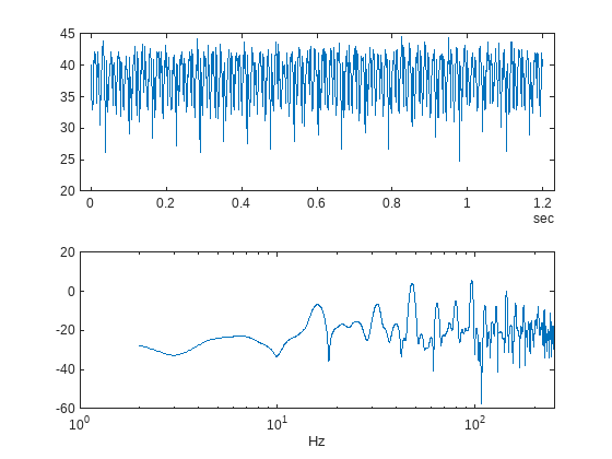
The flow spectrum reveals resonant peaks at expected frequencies. Specifically, the pump motor speed is 950 rpm, or 15.833 Hz, and since the pump has 3 cylinders the flow is expected to have a fundamental at 3*15.833 Hz, or 47.5 Hz, as well as harmonics at multiples of 47.5 Hz. The flow spectrum clearly shows the expected resonant peaks. Faults in one cylinder of the pump will result in resonances at the pump motor speed, 15.833 Hz and its harmonics.
The flow spectrum and slow signal gives some ideas of possible condition indicators. Specifically, common signal statistics such as mean, variance, etc. as well as spectrum characteristics. Spectrum condition indicators relating to the expected harmonics such as the frequency with the peak magnitude, energy around 15.833 Hz, energy around 47.5 Hz, energy above 100 Hz, are computed. The frequency of the spectral kurtosis peak is also computed.
Configure the ensemble with data variables for the condition indicators and condition variables for fault variable values. Then call the extractCI function to compute the features, and use the writeToLastMemberRead command to add the feature and fault variable values to the ensemble. The extractCI function is defined at the end of this example.
ens.DataVariables = [ens.DataVariables; ...
    "fPeak"; "pLow"; "pMid"; "pHigh"; "pKurtosis"; ...
    "qMean"; "qVar"; "qSkewness"; "qKurtosis"; ...
    "qPeak2Peak"; "qCrest"; "qRMS"; "qMAD"; "qCSRange"];
ens.ConditionVariables = ["LeakFault","BlockingFault","BearingFault"];

feat = extractCI(flow,flowP,flowF);
dataToWrite = [faultValues, feat];
writeToLastMemberRead(ens,dataToWrite{:})
The above code preprocesses and computes the condition indicators for the first member of the simulation ensemble. Repeat this for all the members in the ensemble using the ensemble hasdata command. To get an idea of the simulation results under different fault conditions plot every hundredth element of the ensemble.
%Figure with nominal and faults
figure,
subplot(211);
lFlow = plot(flow.Time,flow.Data,'LineWidth',2);
subplot(212);
lFlowP = semilogx(flowF,pow2db(flowP),'LineWidth',2);
xlabel('Hz')
ct = 1;
lColors = get(lFlow.Parent,'ColorOrder');
lIdx = 2;

% Loop over all members in the ensemble, preprocess
% and compute the features for each member
while hasdata(ens)

    % Read member data
    data = read(ens);

    % Preprocess and extract features from the member data
    [flow,flowP,flowF,faultValues] = preprocess(data);
    feat = extractCI(flow,flowP,flowF);

    % Add the extracted feature values to the member data
    dataToWrite = [faultValues, feat];
    writeToLastMemberRead(ens,dataToWrite{:})

    % Plot member signal and spectrum for every 100th member
    if mod(ct,100) == 0
        line('Parent',lFlow.Parent,'XData',flow.Time,'YData',flow.Data, ...
            'Color', lColors(lIdx,:));
        line('Parent',lFlowP.Parent,'XData',flowF,'YData',pow2db(flowP), ...
            'Color', lColors(lIdx,:));
        if lIdx == size(lColors,1)
            lIdx = 1;
        else
            lIdx = lIdx+1;
        end
    end
    ct = ct + 1;
end
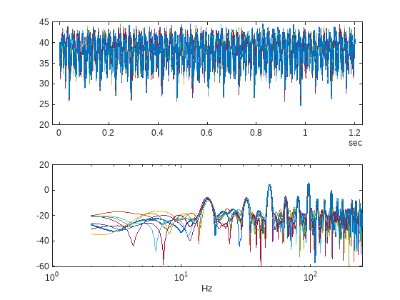
Note that under different fault conditions and severities the spectrum contains harmonics at the expected frequencies.
Detect and Classify Pump Faults
The previous section preprocessed and computed condition indicators from the flow signal for all the members of the simulation ensemble, which correspond to the simulation results for different fault combinations and severities. The condition indicators can be used to detect and classify pump faults from a pump flow signal.
Configure the simulation ensemble to read the condition indicators, and use the tall and gather commands to load all the condition indicators and fault variable values into memory.
% Get data to design a classifier.
reset(ens)
ens.SelectedVariables = [...
    "fPeak","pLow","pMid","pHigh","pKurtosis",...
    "qMean","qVar","qSkewness","qKurtosis",...
    "qPeak2Peak","qCrest","qRMS","qMAD","qCSRange",...
    "LeakFault","BlockingFault","BearingFault"];
idxLastFeature = 14;

% Load the condition indicator data into memory
data = gather(tall(ens));
Evaluating tall expression using the Local MATLAB Session:
- Pass 1 of 1: Completed in 1 min 23 sec
Evaluation completed in 1 min 23 sec
data(1:10,:)
ans=10×17 table
    95.7495      7.4377     96.2464    92.6167    360.9272    38.0157    11.8755    -0.7097    2.9885    19.8385    1.1672    38.1715    2.8614    4.5617e+04    1.0000e-09    0.8000    0
    95.8100      8.7548     76.5278    81.5845    313.7417    38.0201    11.2432    -0.6621    2.8867    19.5544    1.1741    38.1676    2.7860    4.5624e+04    1.0000e-09    0.8000    0
    95.8100      9.3164     95.7408    81.7604    278.1457    38.0174    11.4135    -0.6577    2.8446    17.9044    1.1493    38.1671    2.8103    4.5622e+04    1.0000e-09    0.8000    0
    15.9292    229.8878    172.7189    62.2431    197.8477    35.7389    17.3609    -0.2123    2.2656    19.2586    1.2256    35.9808    3.4465    4.2892e+04    3.2000e-06    0.8000    0
    15.9292    308.9532    176.5983    47.4726    197.8477    35.4528    19.3943    -0.1490    2.1681    19.7606    1.2302    35.7251    3.6708    4.2547e+04    3.6000e-06    0.8000    0
    95.8100     13.8458    112.0437    80.0695    118.3775    37.7084    11.6628    -0.6497    2.8764    19.1244    1.1707    37.8626    2.8293    4.5249e+04    4.0000e-07    0.8000    0
    15.9292    281.9551    180.2683    49.5348    246.6887    35.4056    19.3500    -0.1409    2.1397    18.9874    1.2178    35.6776    3.6818    4.2491e+04    3.6000e-06    0.8000    0
    47.9057    130.4723    147.4706    66.1973    152.3179    36.2711    14.6072    -0.2669    2.3759    17.6148    1.1962    36.4718    3.1342    4.3527e+04    2.4000e-06    0.8000    0
    95.8100      7.1699     98.4639    92.3777    186.2583    38.0051    11.5754    -0.7026    2.8724    18.1011    1.1548    38.1570    2.8239    4.5608e+04    1.0000e-09    0.8000    0
    95.8100     19.4548    107.2855    73.2091    410.5960    37.4699    11.3994    -0.5232    2.4842    16.9398    1.1691    37.6216    2.8115    4.4964e+04    8.0000e-07    0.8000    0
The fault variable values for each ensemble member (row in the data table) can be converted to fault flags and the fault flags combined to single flag that captures the different fault status of each member.
% Convert the fault variable values to flags
data.LeakFlag = data.LeakFault > 1e-6;
data.BlockingFlag = data.BlockingFault < 0.8;
data.BearingFlag = data.BearingFault > 0;
data.CombinedFlag = data.LeakFlag+2*data.BlockingFlag+4*data.BearingFlag;
Create a classifier that takes as input the condition indicators and returns the combined fault flag. Train a support vector machine that uses a 2nd order polynomial kernel. Use the cvpartition command to partition the ensemble members into a set for training and a set for validation.
rng('default') % for reproducibility
predictors = data(:,1:idxLastFeature);
response = data.CombinedFlag;
cvp = cvpartition(size(predictors,1),'KFold',5);

% Create and train the classifier
template = templateSVM(...
    'KernelFunction', 'polynomial', ...
    'PolynomialOrder', 2, ...
    'KernelScale', 'auto', ...
    'BoxConstraint', 1, ...
    'Standardize', true);
combinedClassifier = fitcecoc(...
    predictors(cvp.training(1),:), ...
    response(cvp.training(1),:), ...
    'Learners', template, ...
    'Coding', 'onevsone', ...
    'ClassNames', [0; 1; 2; 3; 4; 5; 6; 7]);
Check the performance of the trained classifier using the validation data and plot the results on a confusion plot.
% Check performance by computing and plotting the confusion matrix
actualValue = response(cvp.test(1),:);
predictedValue = predict(combinedClassifier, predictors(cvp.test(1),:));
confdata = confusionmat(actualValue,predictedValue);
figure,
labels = {'None', 'Leak','Blocking', 'Leak & Blocking', 'Bearing', ...
    'Bearing & Leak', 'Bearing & Blocking', 'All'};
h = heatmap(confdata, ...
    'YLabel', 'Actual leak fault', ...
    'YDisplayLabels', labels, ...
    'XLabel', 'Predicted fault', ...
    'XDisplayLabels', labels, ...
    'ColorbarVisible','off');
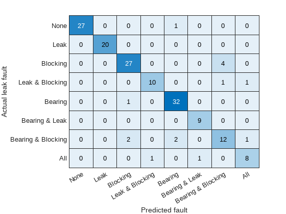
The confusion plot shows for each combination of faults the number of times the fault combination was correctly predicted (the diagonal entries of the plot) and the number of times the fault combination was incorrectly predicted (the off-diagonal entries).
The confusion plot shows that the classifier did not correctly classify some fault conditions (the off diagonal terms). However, the overall validation accuracy was 90% and the accuracy at predicting that there is a fault is 100%.
% Compute the overall accuracy of the classifier
sum(diag(confdata))/sum(confdata(:))
ans = 0.9062
% Compute the accuracy of the classifier at predicting
% that there is a fault
1-sum(confdata(2:end,1))/sum(confdata(:))
ans =
1
Examine the cases where the fault was incorrectly predicted. Find cases in the validation data where the actual fault was a blocking fault but a bearing and blocking fault was predicted.
vData = data(cvp.test(1),:);
b1 = ((actualValue==2) & (predictedValue==6));
fData = vData(b1,15:17)
fData=4×3 table
    1.0000e-09    0.5300    0
    4.0000e-07    0.5900    0
    8.0000e-07    0.7100    0
    4.0000e-07    0.5900    0
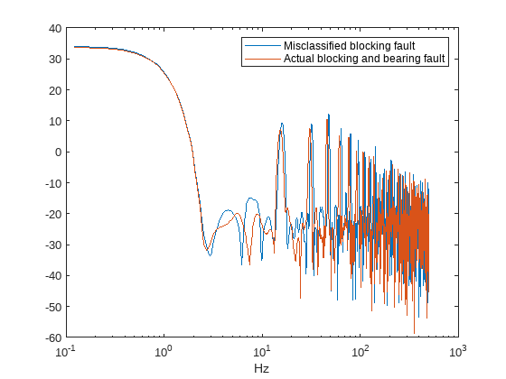
Examining the cases where both bearing and blocking faults was predicted when only a blocking fault did exist reveals that they occur when the leak fault value is close to its nominal value of 1e-9, blocking fault value is around 0.6 and the bearing fault value is at its nominal value of 0. Plotting the spectrum for the case with the fault misclassification and the actual fault, being both bearing and blocking, reveals that spectra are very similar making detection difficult. Using additional pump measurements could provide more information and improve the ability to detect small blocking faults. Alternatively, investigating additional features looking at energy in specific frequency bands can improve the performance.
% Configure the ensemble to only read the flow and fault variable values
ens.SelectedVariables = ["qOut_meas","LeakFault","BlockingFault","BearingFault"];
reset(ens)

% Load the ensemble member data into memory
data = gather(tall(ens));
Evaluating tall expression using the Local MATLAB Session:
- Pass 1 of 1: Completed in 2 min 34 sec
Evaluation completed in 2 min 34 sec
% Look for the member that was incorrectly predicted, and
% compute its power spectrum
idx = ...
    data.BlockingFault == fData.BlockingFault(1) & ...
    data.LeakFault == fData.LeakFault(1) & ...
    data.BearingFault == fData.BearingFault(1);
flow1 = data(idx,1);
flow1 = flow1.qOut_meas{1};
[flow1P,flow1F] = pspectrum(flow1);

% Look for a member that has blocking and bearing faults
idx = ...
    data.BlockingFault == 0.53 & ...
    data.LeakFault == 1e-9 & ...
    data.BearingFault == 6e-4;
flow2 = data(idx,1);
flow2 = flow2.qOut_meas{1};
[flow2P,flow2F] = pspectrum(flow2);

% Plot the power spectra
semilogx(...
    flow1F,pow2db(flow1P),...
    flow2F,pow2db(flow2P));
xlabel('Hz')
legend('Misclassified blocking fault','Actual blocking and bearing fault')
Conclusion
This example showed how to use a Simulink model to model faults in a reciprocating pump, simulate the model under different fault combinations and severities, extract condition indicators from the pump output flow and use the condition indicators to train a classifier to detect pump faults. The example examined the performance of fault detection using the classifier and noted that blocking faults are very similar to the bearing and blocking fault condition and cannot be reliably detected.
Supporting Functions
function [flow,flowSpectrum,flowFrequencies,faultValues] = preprocess(data)
% Helper function to preprocess the logged reciprocating pump data.

% Remove the 1st 0.8 seconds of the flow signal
tMin = seconds(0.8);
flow = data.qOut_meas{1};
flow = flow(flow.Time >= tMin,:);
flow.Time = flow.Time - flow.Time(1);

% Ensure the flow is sampled at a uniform sample rate
flow = retime(flow,'regular','linear','TimeStep',seconds(1e-3));

% Remove the mean from the flow and compute the flow spectrum
fA = flow;
fA.Data = fA.Data - mean(fA.Data);
[flowSpectrum,flowFrequencies] = pspectrum(fA,'FrequencyLimits',[2 250]);

% Find the values of the fault variables from the SimulationInput
simin = data.SimulationInput{1};
vars = {simin.Variables.Name};
idx = strcmp(vars,'leak_cyl_area_WKSP');
LeakFault = simin.Variables(idx).Value;
idx = strcmp(vars,'block_in_factor_WKSP');
BlockingFault = simin.Variables(idx).Value;
idx = strcmp(vars,'bearing_fault_frict_WKSP');
BearingFault = simin.Variables(idx).Value;

% Collect the fault values in a cell array
faultValues = {...
    'LeakFault', LeakFault, ...
    'BlockingFault', BlockingFault, ...
    'BearingFault', BearingFault};
end

function ci = extractCI(flow,flowP,flowF)
% Helper function to extract condition indicators from the flow signal
% and spectrum.

% Find the frequency of the peak magnitude in the power spectrum.
pMax = max(flowP);
fPeak = flowF(flowP==pMax);

% Compute the power in the low frequency range 10-20 Hz.
fRange = flowF >= 10 & flowF <= 20;
pLow = sum(flowP(fRange));

% Compute the power in the mid frequency range 40-60 Hz.
fRange = flowF >= 40 & flowF <= 60;
pMid = sum(flowP(fRange));

% Compute the power in the high frequency range >100 Hz.
fRange = flowF >= 100;
pHigh = sum(flowP(fRange));

% Find the frequency of the spectral kurtosis peak
[pKur,fKur] = pkurtosis(flow);
pKur = fKur(pKur == max(pKur));

% Compute the flow cumulative sum range.
csFlow = cumsum(flow.Data);
csFlowRange = max(csFlow)-min(csFlow);

% Collect the feature and feature values in a cell array.
% Add flow statistic (mean, variance, etc.) and common signal
% characteristics (rms, peak2peak, etc.) to the cell array.
ci = {...
    'qMean', mean(flow.Data), ...
    'qVar',  var(flow.Data), ...
    'qSkewness', skewness(flow.Data), ...
    'qKurtosis', kurtosis(flow.Data), ...
    'qPeak2Peak', peak2peak(flow.Data), ...
    'qCrest', peak2rms(flow.Data), ...
    'qRMS', rms(flow.Data), ...
    'qMAD', mad(flow.Data), ...
    'qCSRange',csFlowRange, ...
    'fPeak', fPeak, ...
    'pLow', pLow, ...
    'pMid', pMid, ...
    'pHigh', pHigh, ...
    'pKurtosis', pKur(1)};
end