Design Input Matching Network for Dipole Antenna
This example shows how to implement an input matching network for a dipole antenna. You can implement the input matching network in three steps:
First, load the precalculated S-parameter matrix for a dipole antenna and the circuit element values of a bandpass filter.
Second, implement a netlist representation of a filter-antenna network using
circuitobjects.Finally, plot the input response and impedance of the network and observe the effect of the matching network.
Load Precalculated Data for Antenna and Bandpass Filter
Load the precalculated S-parameter matrix for a dipole antenna resonating at 850 MHz.
dipole_Sparam = sparameters('Dipole_ant.s1p');Load the precalculated circuit element values of a bandpass filter.
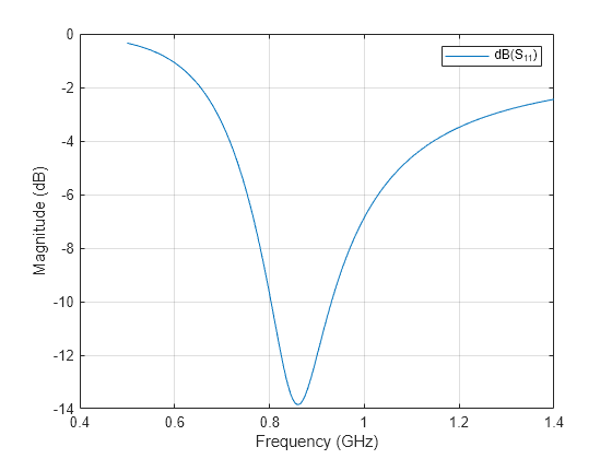
load bpf_elem_dip_ant_matchPlot the S-parameters of the dipole antenna and observe the resonance at 850 MHz.
rfplot(dipole_Sparam)

Set up the frequency sweep parameters.
bw = 200e6; % bandwidth
f0 = 850e6; % center frequency
freq_sweep = f0-2*bw:bw/10000:f0+2*bw;
Implement Netlist Representation of Filter-Antenna Network
Implement a netlist representation of the filter-antenna network using circuit objects. The input matching network is a bandpass filter and its inductor and capacitor values are derived from bpf_elem_dip_ant_match.mat file. The matching network is shown in this figure.

ant = nport(dipole_Sparam);
ant_filt_ckt_1 = circuit('tuned_filt');
add(ant_filt_ckt_1,[1,2],inductor(m01));
add(ant_filt_ckt_1,[2,0],capacitor(c0));
add(ant_filt_ckt_1,[2,3],inductor(ind_bpf(1)));
add(ant_filt_ckt_1,[3,4],capacitor(cap_bpf(1)));
add(ant_filt_ckt_1,[4,0],inductor(ind_bpf(2)));
add(ant_filt_ckt_1,[4,0],capacitor(cap_bpf(2)));
add(ant_filt_ckt_1,[4,5],inductor(ind_bpf(3)));
add(ant_filt_ckt_1,[5,6],capacitor(cap_bpf(3)));
add(ant_filt_ckt_1,[6,0],ant);
Set up the input port for the network analysis.
setports(ant_filt_ckt_1,[1 0],{'in'});
S_ant_filt_1 = sparameters(ant_filt_ckt_1,freq_sweep);
Plot Response of Network
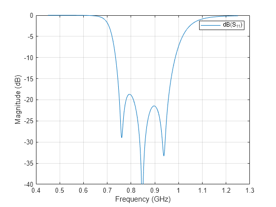
Plot the input response of the network and observe the S11 at the resonance frequency. The operating region of the dipole antenna is widened when it is attached to an input matching network.
figure
rfplot(S_ant_filt_1)
ylim([-40 0])

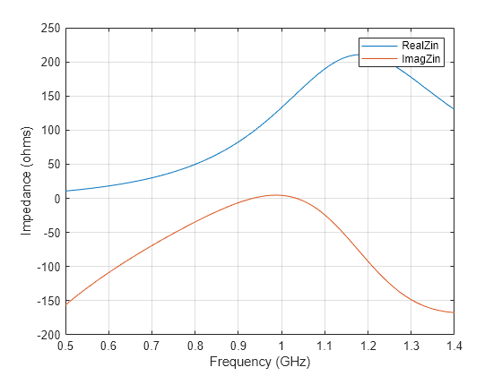
Plot the impedance at the operating region of the dipole antenna.
Z_in_ant = (1+rfparam(dipole_Sparam,1,1))./(1-rfparam(dipole_Sparam,1,1))*50;
figure;
freq = dipole_Sparam.Frequencies;
plot(freq/1e9,real(Z_in_ant))
hold on
plot(freq/1e9,imag(Z_in_ant))
grid on
xlabel('Frequency (GHz)')
ylabel('Impedance (ohms)')
legend('Real{Zin}', 'Imag{Zin}' )
