Matching Network Designer
Description
The Matching Network Designer app lets you design, visualize, and compare matching networks for one-port load.
Using this app, you can:
Design two- and three-component lumped element matching networks at desired frequencies and unloaded-Q factors.
Provide source and load impedance as a one-port Touchstone file, scalar impedance, RF circuit object, RF network parameter object, Antenna Toolbox™ object, or as an anonymous function.
Note
To load one-port circuit object to the app, you must set ports to your circuit object using the
setports
function.To use an Antenna Toolbox object, you must have an Antenna Toolbox license.
One-port Touchstone files include S1P, Z1P, and Y1P file types.
Sort the matching networks using constraints such as operating frequency range and power wave S-parameters.
Plot power wave S-parameters [1] of the matching network on a Smith™ chart and Cartesian plot.
Plot voltage standing wave ratio (VSWR) and impedance transformation plots.
Plot magnitude, phase, real, and imaginary parts of power wave S-parameters of the matching network.
Export selected networks as
circuit
objects or power wave S-parameters assparameters
objects.
More
Available Configurations
The app toolstrip contains these network configurations that you can use to design matching networks:
Pi-Topology
T-Topology
L-Topology
3-Components
Open the Matching Network Designer App
MATLAB® Toolstrip: On the Apps tab, under RF and Mixed-Signal, click the Matching Network Designer app icon.
MATLAB command prompt: Enter
matchingNetworkDesigner
.
Examples
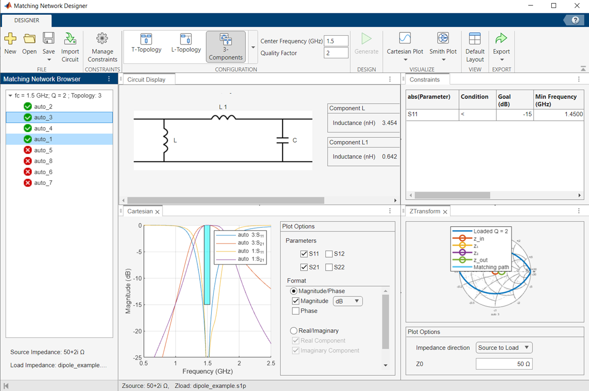
Design, Visualize, and Compare Three-Component Matching Networks
Type this command at the command line to open the Matching Network Designer app.
matchingNetworkDesigner
Select New under File
section to start a new session. In the New Session window, specify the design requirements:
Zs Source —
Scalar Complex Impedance
Impedance (Ohms) —
50+2i
.Zl Source —
Touchstone File
File Name —
dipole_example.s1p
Center Frequency —
1.5e9
andBandwidth —
750e6
.
The app only recognizes one-port Touchstone files and converts the center frequency and bandwidth to Hz.
Select Start session. In the toolstrip of the app window, select 3-Components under the Configuration
section and select Generate to generate the matching network. From the Matching Network Browser pane, select the nodes. For the purpose of this example, select auto_1
. The Quality Factor is populated based on the data entered in the New Session window.
Set constraints to sort the three-component matching networks. To do this, click Manage Constraints. In the Design Constraints window, click button and add the constraints. Set the constraint to:
abs(Parameter) — S11
Condition — <
Goal (dB) — –15
Min Frequency (GHz) — 1.4500
Max Frequency (GHz) — 1.5400
Weight — 1
Select Active and click OK.
The matching networks are sorted based on the constraints and the nodes are rearranged under the Matching Network Browser pane.
Compare the power wave S-parameter results between the nodes. For the purpose of this example, compare the power wave S-parameter results between auto_1
and auto_3
nodes. To do this, select the auto_1
and auto_3
nodes using the Ctrl key. The results are displayed in the Cartesian and Smith plot.
Deselect the auto_3
node. To visualize the impedance transformation of the auto_1
node, select Impedance Transformation under Smith Plot or select the ZTransform
window on the right hand side of the app.
Design Narrow-Band Double Tuning L-Section Matching Network for Monopole Antenna
Design a narrow-band double tuning L-section matching network between a resistive source and a capacitive load in the form of a small monopole. This example designs an L-section matching network consisting of two inductors. The equivalent source impedance is 50
ohms and the load is a monopole with resonant frequency of around 1
GHz. The load (antenna) impedance is at 500
MHz, which is half the resonant frequency.
load_antenna = design(monopole,1e9); sparams_load = sparameters(load_antenna,linspace(0.45e9,0.55e9,101));
To open the Matching Network Designer app, type this command at the command line.
matchingNetworkDesigner
Select New under File
section to start a new session. In the New Session window, specify the requirements:
Zs Source —
Scalar Complex Impedance
Impedance (Ohms) —
50
Zl Source —
S-,Y-, or Z-parameter Object
Variable Name —
sparams_load
Center Frequency —
500e6
andBandwidth —
10e6
.
The app converts the center frequency and bandwidth to Hz.
Select Start Session. In the toolstrip of the app window, select L-Topology under Configuration
section and select Generate to generate the matching network. From the Matching Network Browser pane, select the nodes. For the purpose of this example, select auto_1
.
To plot the VSWR, select VSWR
under Cartesian plot.
Import Custom Matching Network
Design a pi-matching network with circuit objects. For the purpose of this example, the custom pi-matching network consists of two capacitors and an inductor.
Create a circuit
object.
ckt = circuit('test_ckt2');
Create two capacitors, C1
and C2
with the capacitance of 3.35
pF and 2.917
pF.
c1 = capacitor(3.35e-12,'C1'); c2 = capacitor(2.917e-12,'C2');
Create a 5.44
nH inductor.
l = inductor(5.44e-9,'L');
Add C1
to the node [1,0]
of the circuit object.
add(ckt,[1,0],c1);
Add L
to the node [1,2]
of the circuit object.
add(ckt,[1,2],l);
Add C2
to the node [2,0]
of the circuit object.
add(ckt,[2,0],c2);
Save the circuit object.
save('test_file2.mat','ckt');
Set ports to the circuit object and resave the circuit object in MAT file type.
setports(ckt,[1 0],[2 0]); save('test_file2.mat','ckt');
Type this command at the command line to open the Matching Network Designer app.
matchingNetworkDesigner
Select New under File
section to start a new session. In the New Session window, specify the design requirements:
Zs Source —
Scalar Complex Impedance
Impedance (Ohms) —
50
Zl Source —
Touchstone File
File Name —
dipole_example.s1p
Center Frequency —
1.5e9
andBandwidth —
750e6
Select Import Circuit to import the custom pi-matching network designed in this example. Select node test_ckt2
under Matching Network Browser pane.
S11 and S21 plot of the custom pi-matching network is displayed under Cartesian plot.
Related Examples
Programmatic Use
matchingNetworkDesigner
opens the Matching Network
Designer app to design, visualize, and compare one-port narrowband matching
networks.
matchingNetworkDesigner(mnnetwork)
opens a matching network saved
using the Matching Network Designer app. mnnetwork
is a MAT
file.
Tips
Use this expression to set design constraints: |Parameter| Condition 10^(Goal (dB)/20). For example, |S21| > 10^(-3/20) implies that matching network circuits are sorted with
S21
greater than -3
dB as a design constraint. In linear scale the expression can be rewritten as |S21| > 0.7079.
Algorithms
Color Codes in Cartesian Plot
You can use the color codes provided in this table to analyze the Cartesian plot generated in the app. By doing this, you can determine whether your matching network has satisfied the conditions you specified using the Manage Constraints button.
Criteria | S11 and S22 | S12 and S21 |
---|---|---|
Pass | Green | Cyan |
Fail | Orange | Red |
Note
Overlapping regions will result in color mixing.
References
[1] Kurokawa, K. “Power Waves and the Scattering Matrix.” IEEE Transactions on Microwave Theory and Techniques 13, no. 2 (March 1965): 194–202. https://doi.org/10.1109/TMTT.1965.1125964.
[2] Ludwig, Reinhold, and Gene Bogdanov. RF Circuit Design: Theory and Applications. Upper Saddle River, NJ: Prentice-Hall, 2009.
Version History
Introduced in R2021a
MATLAB Command
You clicked a link that corresponds to this MATLAB command:
Run the command by entering it in the MATLAB Command Window. Web browsers do not support MATLAB commands.
Select a Web Site
Choose a web site to get translated content where available and see local events and offers. Based on your location, we recommend that you select: .
You can also select a web site from the following list
How to Get Best Site Performance
Select the China site (in Chinese or English) for best site performance. Other MathWorks country sites are not optimized for visits from your location.
Americas
- América Latina (Español)
- Canada (English)
- United States (English)
Europe
- Belgium (English)
- Denmark (English)
- Deutschland (Deutsch)
- España (Español)
- Finland (English)
- France (Français)
- Ireland (English)
- Italia (Italiano)
- Luxembourg (English)
- Netherlands (English)
- Norway (English)
- Österreich (Deutsch)
- Portugal (English)
- Sweden (English)
- Switzerland
- United Kingdom (English)
Asia Pacific
- Australia (English)
- India (English)
- New Zealand (English)
- 中国
- 日本Japanese (日本語)
- 한국Korean (한국어)