System with Uncertain Parameters
As an example of a closed-loop system with uncertain parameters, consider the two-cart "ACC Benchmark" system [13] consisting of two frictionless carts connected by a spring shown as follows.
ACC Benchmark Problem
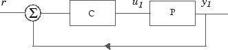
The system has the block diagram model shown below, where the individual carts have the respective transfer functions.
The parameters m1, m2, and k are uncertain, equal to one plus or minus 20%:
m1 = 1 ± 0.2
m2 = 1 ± 0.2
k = 1 ± 0.2
"ACC Benchmark" Two-Cart System Block Diagram y1 = P(s) u1
The upper dashed-line block has transfer function matrix F(s):
Build the Uncertain Model
To build the uncertain model of the ACC Benchmark two-cart system, first create uncertain real parameters for the masses and spring constant.
m1 = ureal('m1',1,'percent',20);
m2 = ureal('m2',1,'percent',20);
k  = ureal('k',1,'percent',20);
Next, create the transfer functions for each cart.
s = zpk('s');
G1 = ss(1/s^2)/m1;
G2 = ss(1/s^2)/m2;
Use model arithmetic to assemble F(s), and connect F(s) to the spring k.
F = [0;G1]*[1 -1]+[1;-1]*[0,G2];
P = lft(F,k)
Uncertain continuous-time state-space model with 1 outputs, 1 inputs, 4 states.
The model uncertainty consists of the following blocks:
  k: Uncertain real, nominal = 1, variability = [-20,20]%, 1 occurrences
  m1: Uncertain real, nominal = 1, variability = [-20,20]%, 1 occurrences
  m2: Uncertain real, nominal = 1, variability = [-20,20]%, 1 occurrences
Model Properties

Type "P.NominalValue" to see the nominal value and "P.Uncertainty" to interact with the uncertain elements.
The resulting P is a SISO uncertain state-space (uss) object with four states and three uncertain parameters, m1, m2, and k. You can obtain the nominal plant from the NominalValue property.
Pnom = zpk(P.NominalValue)
Pnom =

        1
  -------------
  s^2 (s^2 + 2)

Continuous-time zero/pole/gain model.
Model Properties
Suppose that the uncertain model P(s) has a negative feedback controller with the following transfer function.
Form the closed-loop transfer function from r to y1 with P(s) and P(s) in the standard configuration.
C = 100*ss((s+1)/(.001*s+1))^3;
T = feedback(P*C,1);
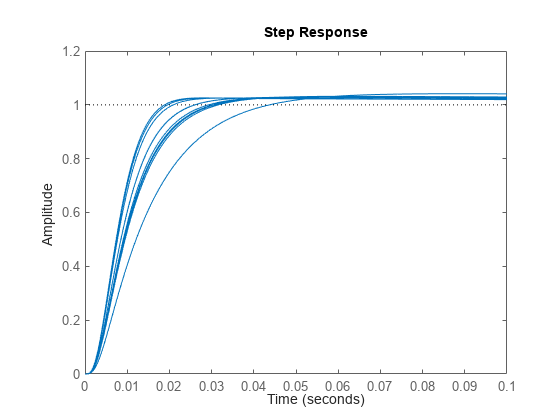
View the closed-loop step response on the time interval from t = 0 s to t = 0.1 s. Use usample to generate Monte Carlo random samples of ten combinations of the three uncertain parameters and plot the response. The result gives a sense of the range of responses and the robustness of the system against variations in the uncertain values.
stepplot(usample(T,10),.1);