Main Content

ncfmr

(Not recommended) Model reduction from normalized coprime factorization

ncfmr is not recommended. Use reducespec instead. (since R2023b) For more information on updating your code, see Version History.

Description

ncfmr computes a reduced-order approximation of a model by truncating modes in a coprime factorization of the full-order model. This method is related to the balanced truncation method, but it is particularly well-suited to controller order reduction. For a stabilizing controller, the reduced controller is also stabilizing as long as the approximation error is smaller than the robustness margin computed by ncfmargin.

example

[Gred,info] = ncfmr(G,ord) computes a reduced-order approximation of the dynamic system model G. Specify the desired reduction order as ord. If ord is a vector, then Gred is an array of approximations of the corresponding order. The structure info contains information about the computation such as bounds on the approximation error.

[~,info] = ncfmr(G) computes the coprime factorization of G given by [M,N] such that G = M\N (see lncf), the Hankel singular values of the factorization, and the error bounds. You can use this information to determine the target reduction order programmatically based on desired fidelity or robust stability considerations. Then, use the syntax Gred = ncfmr(G,ord,info) to compute the reduced-order model.

Gred = ncfmr(G,ord,info) computes the reduced-order approximation using the normalized coprime factorization and Hankel singular values that you provide in info. Obtain info using the previous syntax, [~,info] = ncfmr(G). Providing a previously computed info to ncfmr allows you to perform model reduction without having to recompute the factorization and Hankel singular values. This syntax is therefore particularly useful when performance is a concern.

example

ncfmr(G) plots the Hankel singular values and bounds on the approximation error corresponding to each order. Examine the plot to determine a reduced order based on desired fidelity or robust stability considerations. You can then use Gred = ncfmr(G,ord) to compute the reduced-order model.

Examples

collapse all

ncfmr computes Hankel singular values and approximation errors to help you select a suitable target reduction order. One way to do so is to examine a plot of these values. Suppose that you have a data file ncfmrModel.mat containing the 30-state plant model G.

load("ncfmrModel.mat","G")
size(G)
State-space model with 2 outputs, 3 inputs, and 30 states.

Call ncfmr without an output argument. The function generates a Hankel singular value plot, which shows the relative energy contributions of each state in the coprime factorization of G, arranged in decreasing order by energy. The plot also shows the upper bound on the error between the original and reduced-order models that you obtain by truncating the states at that point. Examine this plot to choose the target order. For instance, for a maximum error of 0.01, you can reduce the model to 13th order.

ncfmr(G)

Call ncfmr again with an output argument and using order = 13. Doing so computes the reduced model Gred. Examine the singular values of G and of the difference between G and Gred. The difference is very small across all frequencies, showing that the reduced-order model is a good approximation of the full-order model.

Gred = ncfmr(G,13);
sigma(G,G-Gred)
legend("G","G-Gred")

Input Arguments

collapse all

Model to reduce, specified as a dynamic system model such as a state-space (ss) model. G can be stable or unstable. If G is a generalized state-space model with uncertain or tunable control design blocks, then the function uses the nominal or current value of those elements. sys cannot be an frd model or a model with time delays.

Reduction order, specified as a positive integer or a vector of positive integers. If ord is a scalar, ncfmr returns the model Gred of that order. If ord is a vector, then Gred is an array of models reduced to the corresponding orders.

To determine ord, you can use one of two methods:

  • Use the syntax ncfmr(G) to obtain a plot of Hankel singular values and bounds on approximation errors at each order. Examine the plot to choose a reduction order with a tolerable approximation error. For an example, see Reduce Model Order.

  • Use the syntax [~,info] = ncfmr(G) to obtain the info structure. Programmatically examine the approximation error bounds in info.ErrorBounds to choose a reduction order.

If G has unstable states, then ord must be at least the number of unstable states.

Output Arguments

collapse all

Reduced-order model, returned as a state-space (ss) model. If ord is a scalar, then Gred is a single model of order ord. If ord is a vector, then Gred is an array of ss models of corresponding orders.

Information about model-reduction calculation, returned as a structure with the following fields.

  • GL — Left normalized coprime factorization of G, returned as a state-space (ss) model. This factorization is given by GL = lncf(G). For more information, see lncf.

  • HSV — Hankel singular values of GL, returned as a vector whose length is the number of states in G. These values indicate the relative energy contribution of each state. You can choose a target reduction order by examining these values and choosing a number of states after which the energy contribution drops off significantly.

  • ErrorBound — Upper bound on approximation errors, returned as a vector. The approximation error is given by [Mr,Nr][M,N], where [M,N] = lncf(G) and [Mr,Nr] = lncf(Gred). (For more information about these expressions, see lncf.) Each entry info.ErrorBound(j) is the maximum approximation error associated with reducing to j states. Thus, for instance, if you want an approximation error of no more than 0.01, examine info.ErrorBound to find the index of the first entry that is less than 0.01. Use that index as ord.

Tips

  • You can use ncfmr to reduce the plant G or controller K while preserving closed-loop stability of the following SISO or MIMO feedback loop.
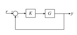
    Feedback loop formed by controller K and plant G with negative unit feedback, feedback(G*K,eye(n)).

    Stability of this loop is preserved as long as the approximation error of the reduced plant is smaller than the robustness margin for this loop given by ncfmargin(G,K).

    For controllers computed with ncfsyn, reducing the controller Ks that ncfsyn computes for the shaped controller Gs is preferable. Both Ks and Gs are returned by ncfsyn in the info output argument. You can then compute Kr, the reduced controller for the original plant G, from Kr = W1KsrW2, where W1 and W2 are the shaping weights used with ncfsyn.

    For controllers obtained by other techniques, reduction with ncfmr also preserves stability if the error does not exceed the ncfmargin margin. However, such reduction can partially remove integral action and introduce steady-state tracking errors. Therefore, removing any integrator terms from the controller before reduction with ncfmr and replacing them in the reduced controller is recommended.

Algorithms

ncfmr performs the following steps to reduce the input model G to the desired order k.

  1. Find the left normalized coprime factorization [M,N] of G, where G = M\N (see lncf).

  2. Obtain the kth-order approximation [Mr,Nr] of [M,N], using balanced model truncation with absolute error control.

  3. Set Gred = Mr\Nr.

Version History

Introduced before R2006a

expand all

R2023b: Not recommended

ncfmr is not recommended. To perform balanced truncation of normalized coprime factors, use the reducespec function with this syntax.

R = reducespec(sys,"ncf");

For the full workflow, see Task-Based Model Order Reduction Workflow.