Bias and Variability in the Periodogram
This example shows how to reduce bias and variability in the periodogram. Using a window can reduce the bias in the periodogram, and using windows with averaging can reduce variability.
Use wide-sense stationary autoregressive (AR) processes to show the effects of bias and variability in the periodogram. AR processes present a convenient model because their PSDs have closed-form expressions. Create an AR(2) model of the following form:
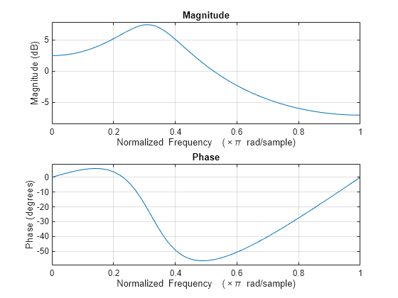
where is a zero mean white noise sequence with some specified variance. In this example, assume the variance and the sampling period to be 1. To simulate the preceding AR(2) process, create an all-pole (IIR) filter. View the magnitude response of the filter.
B2 = 1;
A2 = [1 -0.75 0.5];
freqz(B2,A2)

This process is bandpass. The dynamic range of the PSD is approximately 14.5 dB, as you can determine with the following code.
[H2,W2] = freqz(B2,A2);
dr2 = max(mag2db(abs(H2)))-min(mag2db(abs(H2)))
dr2 =
14.4982
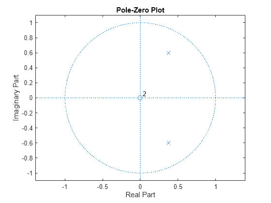
By examining the placement of the poles, you see that this AR(2) process is stable. The two poles are inside the unit circle.
zplane(B2,A2)

Next, create an AR(4) process described by the following equation:
Use the following code to view the magnitude response of this IIR system.
B4 = 1;
A4 = [1 -2.7607 3.8106 -2.6535 0.9238];
freqz(B4,A4)

Examining the placement of the poles, you can see this AR(4) process is also stable. The four poles are inside the unit circle.
zplane(B4,A4)

The dynamic range of this PSD is approximately 65 dB, much larger than the AR(2) model.
[H4,W4] = freqz(B4,A4);
dr4 = max(mag2db(abs(H4)))-min(mag2db(abs(H4)))
dr4 =
64.6343
To simulate realizations from these AR(p) processes, use randn and filter. Set the random number generator to the default settings to produce repeatable results. Plot the realizations.
rng default
x = randn(1e3,1);
y2 = filter(B2,A2,x);
y4 = filter(B4,A4,x);

subplot(2,1,1)
plot(y2)
title("AR(2) Process")
xlabel("Time")

subplot(2,1,2)
plot(y4)
title("AR(4) Process")
xlabel("Time")

Compute and plot the periodograms of the AR(2) and AR(4) realizations. Compare the results against the true PSD.
subplot(2,1,1)
periodogram(y2)
hold on
plot(W2/pi,mag2db(abs(H2)/sqrt(pi)))
title("AR(2) PSD and Periodogram")
hold off

subplot(2,1,2)
periodogram(y4)
hold on
plot(W4/pi,mag2db(abs(H4)/sqrt(pi)))
title("AR(4) PSD and Periodogram")
text(0.6,10,"\downarrow Bias")
hold off

In the case of the AR(2) process, the periodogram estimate follows the shape of the true PSD but exhibits considerable variability. This is due to the low degrees of freedom. The pronounced negative deflections (in dB) in the periodogram are explained by taking the log of a chi-square random variable with two degrees of freedom.
In the case of the AR(4) process, the periodogram follows the shape of the true PSD at low frequencies but deviates from the PSD in the high frequencies. This is the effect of the convolution with Fejér's kernel. The large dynamic range of the AR(4) process compared to the AR(2) process is what makes the bias more pronounced.
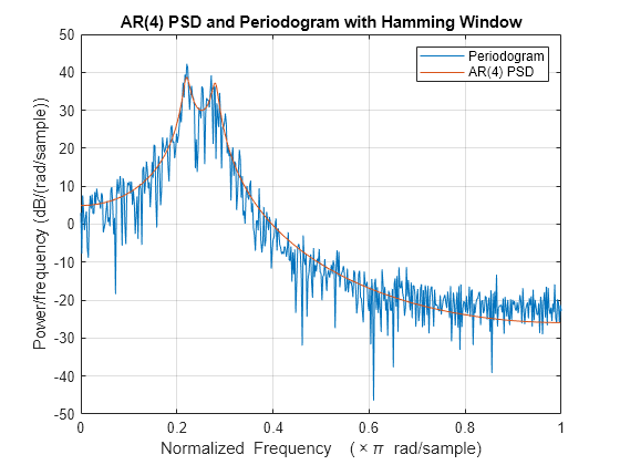
Mitigate the bias demonstrated in the AR(4) process by using a taper, or window. In this example, use a Hamming window to taper the AR(4) realization before obtaining the periodogram.
figure
periodogram(y4,hamming(length(y4)))
hold on
plot(W4/pi,mag2db(abs(H4)/sqrt(pi)))
title("AR(4) PSD and Periodogram with Hamming Window")
legend("Periodogram","AR(4) PSD")
hold off

Note that the periodogram estimate now follows the true AR(4) PSD over the entire Nyquist frequency range. The periodogram estimates still only have two degrees of freedom so the use of a window does not reduce the variability of periodogram, but it does address bias.
In nonparametric spectral estimation, two methods for increasing the degrees of freedom and reducing the variability of the periodogram are Welch's overlapped segment averaging and multitaper spectral estimation.
Obtain a multitaper estimate of the AR(4) time series using a time half bandwidth product of 3.5. Plot the result.
NW = 3.5;

pmtm(y4,NW)
hold on
plot(W4/pi,mag2db(abs(H4)/sqrt(pi)))
legend("Multitaper Estimate","AR(4) PSD")
hold off

The multitaper method produces a PSD estimate with significantly less variability than the periodogram. Because the multitaper method also uses windows, you see that the bias of the periodogram is also addressed.