Solver
Solver that computes states and outputs for simulation
Model Configuration Pane: Solver
Description
The Solver parameter specifies the solver that computes the states of the model during simulation and in generated code. In the process of solving the set of ordinary differential equations that represent the system the model implements, the solver also determines the next time step for the simulation.
When you enable the Use local solver when referencing model parameter for a referenced model, the Solver parameter for the referenced model specifies the solver to use as a local solver. The local solver solves the referenced model as a separate set of differential equations. For more information, see Use Local Solvers in Referenced Models.
The software provides several types of fixed-step and variable-step solvers.
Variable-Step Solvers
A variable-step solver adjusts the interval between simulation time hits where the solver computes states and outputs based on the system dynamics and specified error tolerance. For most variable-step solvers, you can configure additional parameters, including:
Fixed-Step Solvers
In general, fixed-step solvers except for ode14x and
ode1be calculate the next step using this formula:
X(n+1) = X(n) + h dX(n)
where X is the state, h is the step size, and dX is the state derivative. dX(n) is calculated by a particular algorithm using one or more derivative evaluations depending on the order of the method.
For most fixed-step solvers, you can configure additional parameters, including:
Settings
auto (Automatic solver selection) (default) | discrete (no continuous states) | ...In general, the automatic solver selection chooses an appropriate solver for each model. The choice of solver depends on several factors, including the system dynamics and the stability of the solution. For more information, see Choose a Solver.
The options available for this parameter depend on the value you select for the solver Type.
auto (Automatic solver selection)The software selects the variable-step solver to compute the model states based on the model dynamics. For most models, the software selects an appropriate solver.
discrete (no continuous states)Use this solver only for models that contain no states or only discrete states. The
discretevariable-step solver computes the next simulation time hit by adding a step size that depends on the rate of change for states in the model.ode45 (Dormand-Prince)When you manually select a solver,
ode45is an appropriate first choice for most systems. Theode45solver computes model states using an explicit Runge-Kutta (4,5) formula, also known as the Dormand-Prince pair, for numerical integration.ode23 (Bogacki-Shampine)The
ode23solver computes the model states using an explicit Runge-Kutta (2,3) formula, also known as the Bogacki-Shampine pair, for numerical integration.For crude tolerance and in the presence of mild stiffness, the
ode23solver is more efficient than theode45solver.ode113 (Adams)The
ode113solver computes the model states using a variable-order Adams-Bashforth-Moulton PECE numerical integration technique.The
ode113solver uses the solutions from several preceding time points to compute the current solution.The
ode113solver can be more efficient thanode45for stringent tolerances.ode15s (stiff/NDF)The
ode15ssolver computes the model states using variable-order numerical differentiation formulas (NDFs). NDFs are related to but more efficient than the backward differentiation formulas (BDFs), also known as Gear's method.The
ode15ssolver uses the solutions from several preceding time points to compute the current solution.The
ode15ssolver is efficient for stiff problems. Try this solver if theode45solver fails or is inefficient.ode23s (stiff/Mod. Rosenbrock)The
ode23ssolver computes the model states using a modified second-order Rosenbrock formula.The
ode23ssolver uses only the solution from the preceding time step to compute the solution for the current time step.The
ode23ssolver is more efficient than theode15ssolver for crude tolerances and can solve stiff problems for whichode15sis ineffective.ode23t (mod. stiff/Trapezoidal)The
ode23tsolver computes the model states using an implementation of the trapezoidal rule.The
ode23tsolver uses only the solution from the preceding time step to compute the solution for the current time step.Use the
ode23tsolver for problems that are moderately stiff and require a solution with no numerical damping.ode23tb (stiff/TR-BDF2)The
ode23tbsolver computes the model states using a multistep implementation of TR-BDF2, an implicit Runge-Kutta formula with a trapezoidal rule first stage and a second stage that consists of a second-order backward differentiation formula. By construction, the same iteration matrix is used in both stages.The
ode23tbsolver is more efficient thanode15sfor crude tolerances and can solve stiff problems for which theode15ssolver is ineffective.odeN (Nonadaptive)The
odeNsolver uses a nonadaptive fixed-step integration formula to compute the model states as an explicit function of the current value of the state and the state derivatives approximated at intermediate points.The nonadaptive
odeNsolver does not adjust the simulation step size to satisfy error constraints but does reduce step size in some cases for zero-crossing detection and discrete sample times.daessc (DAE solver for Simscape™)The
daesscsolver computes the model states by solving systems of differential algebraic equations modeled using Simscape. Thedaesscsolver provides robust algorithms specifically designed to simulate differential algebraic equations that arise from modeling physical systems.The
daesscsolver is available only with Simscape products.
auto (Automatic solver selection)The software selects a fixed-step solver to compute the model states based on the model dynamics. For most models, the software selects an appropriate solver.
discrete (no continuous states)Use this solver only for models that contain no states or only discrete states. The
discretefixed-step solver relies on blocks in the model to update discrete statesThe discrete fixed-step solver does not support zero-crossing detection.
ode8 (Dormand-Prince)The
ode8solver uses the eighth-order Dormand-Prince formula to compute the model state as an explicit function of the current value of the state and the state derivatives approximated at intermediate points.ode5 (Dormand-Prince)The
ode5solver uses the fifth-order Dormand-Prince formula to compute the model state as an explicit function of the current value of the state and the state derivatives approximated at intermediate points.ode4 (Runge-Kutta)The
ode4solver uses the fourth-order Runge-Kutta (RK4) formula to compute the model state as an explicit function of the current value of the state and the state derivatives.ode3 (Bogacki-Shampine)The
ode3solver computes the state of the model as an explicit function of the current value of the state and the state derivatives. The solver uses the Bogacki-Shampine Formula integration technique to compute the state derivatives.ode2 (Heun)The
ode2solver uses the Heun integration method to compute the model state as an explicit function of the current value of the state and the state derivatives.ode1 (Euler)The
ode1solver uses the Euler integration method to compute the model state as an explicit function of the current value of the state and the state derivatives. This solver requires fewer computations than a higher order solver but provides comparatively less accuracy.ode14x (extrapolation)The
ode14xsolver uses a combination of Newton's method and extrapolation from the current value to compute the model state as an implicit function of the state and the state derivative at the next time step. In this example, X is the state, dX is the state derivative, and h is the step size:X(n+1) - X(n)- h dX(n+1) = 0
This solver requires more computation per step than an explicit solver but is more accurate for a given step size.
ode1be (Backward Euler)The
ode1besolver is a Backward Euler type solver that uses a fixed number of Newton iterations and incurs a fixed computational cost. You can use theode1besolver as a computationally efficient fixed-step alternative to theode14xsolver.
Examples
Open the model vdp.
mdl = "vdp";
open_system(mdl)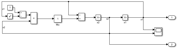
To allow the software to select the solver to use for the model, specify the Type parameter as Fixed-step or Variable-step, and set the Solver parameter to auto. For this example, configure the software to select a variable-step solver for the model.
To open the Configuration Parameters dialog box, on the Modeling tab, click Model Settings.
On the Solver pane, set the solver Type to
Variable-stepand the Solver parameter toauto (Automatic solver selection).Click OK.
Alternatively, use the set_param function to set the parameter values programmatically.
set_param(mdl,"SolverType","Variable-step", ...
    "SolverName","VariableStepAuto")
Simulate the model. On the Simulation tab, click Run. Alternatively, use the sim function.
out = sim(mdl);
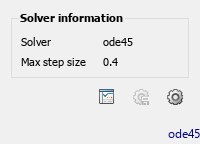
As part of initializing the simulation, the software analyzes the model to select the solver. The status bar on the bottom of the Simulink Editor indicates the selected solver on the right. For this model, the software selects the ode45 solver.
![]()
To view more information about the selected solver parameters, click the text in the status bar that indicates the selected solver. The Solver Information menu shows the selected solver and the selected value for the Max step size parameter. For this simulation, the solver uses a maximum step size of 0.4.

If you want to lock down the solver selection and maximum step size, explicitly specify the solver parameter values. In the Solver information menu, click Accept suggested settings ![]() .
.
Alternatively, you can use the set_param function to specify the parameter values programmatically.
set_param(mdl,"SolverName","ode45","MaxStep","0.4")
After you explicitly specify the parameter values, the solver information in the status bar and Solver information menu no longer indicate that the parameter values are automatically selected.
Tips
The optimal solver balances acceptable accuracy with the shortest simulation time. Identifying the optimal solver for a model requires experimentation. For more information, see Choose a Solver.
When you use fast restart, you can change the solver for the simulation without having to recompile the model. (since R2021b)
The software uses a discrete solver for models that have no states or have only discrete states, even if you specify a continuous solver.
Programmatic Use
Parameter: SolverName or Solver |
| Type: string | character vector |
Variable-Step Solver Values:
"VariableStepAuto" | "VariableStepDiscrete" |
"ode45" | "ode23" |
"ode113" | "ode15s" |
"ode23s" | "ode23t" |
"ode23tb" | "odeN" |
"daessc" |
Fixed-Step Solver Values:
"FixedStepAuto" | "FixedStepDiscrete" |
"ode8" | "ode5" |
"ode4" | "ode3" |
"ode2" | "ode1" |
"ode14x" | "ode1be" |
Default:
"VariableStepAuto" |
Version History
Introduced before R2006a