Frequency Response Estimation for Permanent Magnet Synchronous Motor Model
This example shows the frequency response estimation workflow for a Field-Oriented Controlled (FOC) three-phase Permanent Magnet Synchronous Motor (PMSM) modeled using components from Motor Control Blockset™. This example uses Model Linearizer from Simulink® Control Design™ software to obtain a frequency-response model (frd) object, which you can use to estimate a parametric model for the motor.
PMSM Model
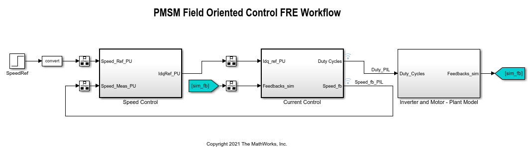
The PMSM model is based on the Motor Control Blockset mcb_pmsm_foc_sim model. The model includes:
A subsystem to model inverter and PMSM dynamics
Inner-loop (current) and outer-loop (speed) PI controllers to implement a field-oriented control algorithm for motor speed control
You can examine this model for more details. In this example, the original model is modified to ensure that the simulation starts from a steady state. The steady state serves as the operating point used in the frequency response estimation workflow.
Open the Simulink model.
model = 'scd_fre_mcb_pmsm_foc_sim';
open_system(model)
Modify Model to Start Simulation from Steady State
To ensure that the simulation starts from a steady state, modify initial conditions of the original model. To obtain these initial conditions, enable signal logging for the speed feedback signal and simulate the model to the steady state, with a speed of 0.5 per-unit (p.u.). To ensure that the speed reaches the desired steady state, after the simulation, examine the simulation result in the Simulation Data Inspector.
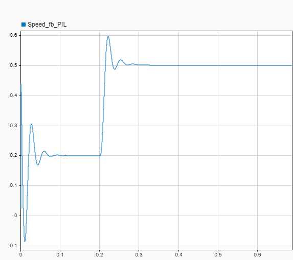
Based on the speed response in the preceding figure, you can use the simulation results after 0.6 seconds to obtain block initial conditions for frequency response estimation. In addition to the initial conditions, modify settings in filters associated with the speed control loop for faster speed reference tracking. The changes are intended to make the simulation start from a steady state but do not affect the motor plant model. Make the following changes to the model.
In the SpeedRef block, set Step time to
0s and Initial value to the steady state reference value0.5p.u.In the Speed Control subsystem, in the Zero_Cancellation block, set Filter coefficient to
1for faster tracking.In the Speed Control > PI_Controller_Speed subsystem, in the Ki2 block, set the Constant value to
0.01725. That is, the speed controller's initial value,y0.In the Current Control > Input Scaling > Calculate Position and Speed subsystem, in the Speed Measurement block, set the Delays for speed calculation to
1for faster speed measurement.In the Current Control > Control_System > Closed Loop Control > Current_Controllers > PI_Controller_Id subsystem, in the Ki1 block, set the Constant value to
0.025. That is, d-axis controller's initial value,y0.In the Current Control > Control_System > Closed Loop Control > Current_Controllers > PI_Controller_Iq subsystem, in the Kp1 block, set the Constant value to
0.435. That is, q-axis controller's initial value,y0.In Inverter and Motor - Plant Model subsystem, in the Surface Mount PMSM block, set Initial d-axis and q-axis current (idq0) to
[-0.4 0.55]and Initial rotor mechanical speed (omega_init) to215.
Alternatively, you can set the block parameters using the following commands.
set_param([model,'/SpeedRef'],'Time','0','Before','0.5')
set_param([model,'/Speed Control/Zero_Cancellation'],'Filter_constant','1')
set_param([model,'/Speed Control/PI_Controller_Speed/Ki2'],'Value','0.01725')
set_param([model,...
    '/Current Control/Input Scaling/ Calculate Position and Speed/Speed Measurement'],...
    'DelayLength','1')
currCtrlsPath = '/Current Control/Control_System/Closed Loop Control/Current_Controllers/';
set_param([model,currCtrlsPath,'PI_Controller_Id/Ki1'],'Value','0.025')
set_param([model,currCtrlsPath,'PI_Controller_Iq/Kp1'],'Value','0.435')
set_param([model,'/Inverter and Motor - Plant Model/Surface Mount PMSM'], ...
    'idq0','[-0.4 0.55]','omega_init','215')
Frequency Response Estimation Using Fixed Sample Sinestream Signal
After the necessary changes, the simulation starts from a steady state with the motor speed around 0.5 p.u. You can then use Model Linearizer to conduct frequency response estimation. To open the Model Linearizer, in the Simulink model window, in the Apps gallery, click Model Linearizer.
To collect frequency response data, you must first specify the portion of model to estimate. By default, Model Linearizer uses the linearization analysis points defined in the model (the model I/Os) to determine where to inject the test signal and where to measure the frequency response. The model scd_fre_mcb_pmsm_foc_sim contains predefined linear analysis points:
Open-loop input points at the outputs of d-axis and q-axis current PI controllers
Open-loop output points at speed, d-axis current, and q-axis current feedback signals
To view or edit these analysis points, on the Estimation tab of Model Linearizer, on the Analysis I/Os list, click Edit Model I/Os. Analysis points for estimation work the same way as analysis points for linearization. For more information about linear analysis points, see Specify Portion of Model to Linearize.
Additionally, find all source blocks in the signal paths of the linearization outputs that generate time-varying signals. Such time-varying signals can interfere with the signal at the linearization output points and produce inaccurate estimation results. To disable the time-varying source blocks, click More Options. In the Options for frequency response estimation dialog box, on the Time Varying Sources tab, click Find and add time varying source blocks automatically.
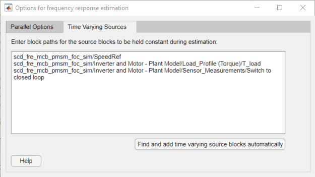
The software holds the values of these blocks at their corresponding initial conditions during frequency response estimation.
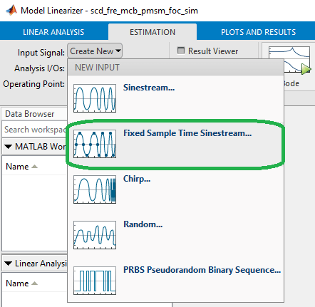
For this example, create a fixed sample time sinestream input signal for estimation. Create a signal with 20 frequency points from 1 rad/s to 2000 rad/s and an amplitude of 0.05. For more information on defining sinestream input signals, see Sinestream Input Signals.
To create the signal, on the Estimation tab of the Model Linearizer, in the Input Signal list, select Fixed Sample Time Sinestream.
In the Specify fixed sample time dialog box, specify a Sample time of 5e-5 seconds.
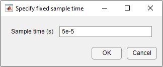
Click OK. The Create sinestream input with fixed sample time dialog box opens.
Specify the frequency units for estimation. In the Frequency units list, select rad/s.
To specify the frequencies at which to estimate the plant response, click the add frequencies icon.
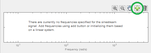
In the Add frequencies dialog box, specify 20 logarithmically spaced frequencies ranging from 1 rad/s to 2000 rad/s.
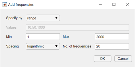
Click OK. The added points are visible in the frequency content viewer of the Create sinestream input with fixed sample time dialog box.
To specify the amplitude of the input signal, first select all the frequencies in the plot area. Then, in the Amplitude field, enter 0.05. Use default values for the remaining parameters.
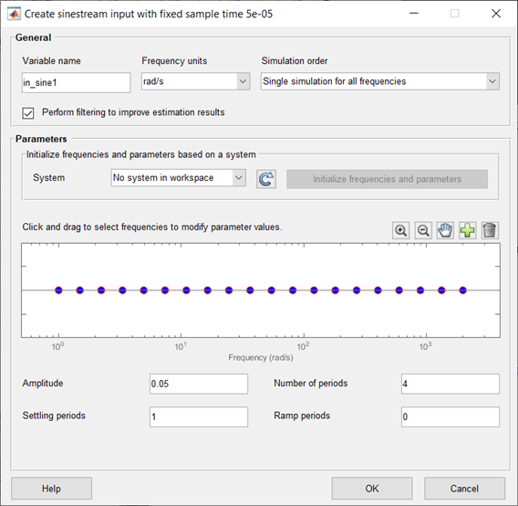
Click OK to create the fixed sample time sinestream signal.
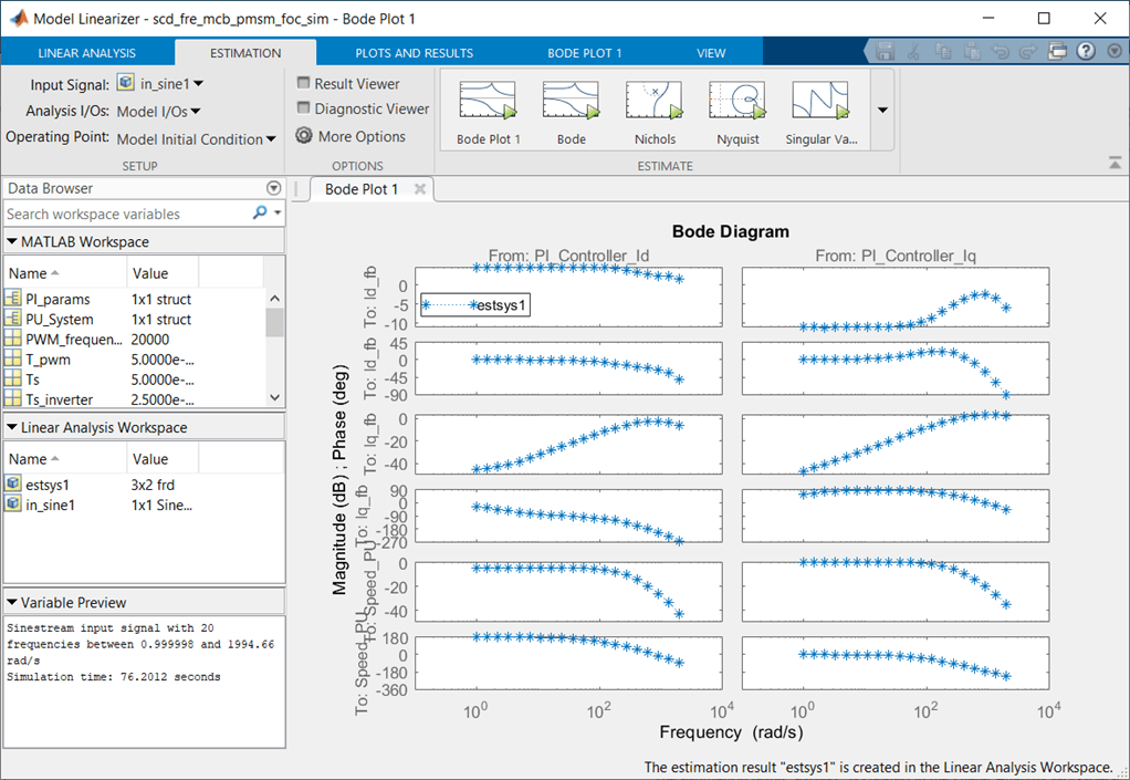
To estimate and plot the frequency response, one the Estimation tab, click Bode. The estimated frequency response appears in the Linear Analysis Workspace as the frd model estsys1 and response is added to Bode Plot 1.
Frequency Response Estimation Using PRBS Input Signal
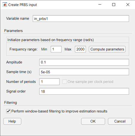
In addition to sinestream input signals, you can also use PRBS input signals in frequency response estimation. For this example, create an input signal with 1 period, an order of 18, and an amplitude of 0.1.
To create the signal, on the Estimation tab of the Model Linearizer, in the Input Signal list, click PRBS Pseudorandom Binary Sequence.
In the Create PRBS input dialog box, configure the parameters of the PRBS signal. The input dialog box assists you to set the signal order and number of periods based on the frequency range you are interested in. First, set the Sample time to 5e-5 seconds. Next, enter a frequency range between 1 rad/s and 2000 rad/s, and then click Compute Parameters. The software computes the signal parameters Number of periods and Signal order. To ensure that the system is properly excited, set the perturbation amplitude to 0.1 using the Amplitude parameter. Use default values for the remaining parameters.
Click OK to create the input signal.
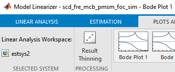
To estimate and plot the frequency response, on the Estimation tab, click Bode. The estimated frequency response appears in the Linear Analysis Workspace as the frd model estsys2. Frequency response estimation with PRBS input signal produces results with a large number of frequency points. You can use the Result Thinning functionality to extract an interpolated result from an estimated frequency response model across a specified frequency range and number of frequency points.
To apply thinning to the estimated result, select estsys2 in the Linear Analysis Workspace, and on the Plots and Results tab click Result Thinning.
In the Specify frequencies dialog box, specify a frequency range between 1 rad/s and 2000 rad/s with 30 logarithmically spaced points.
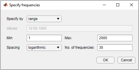
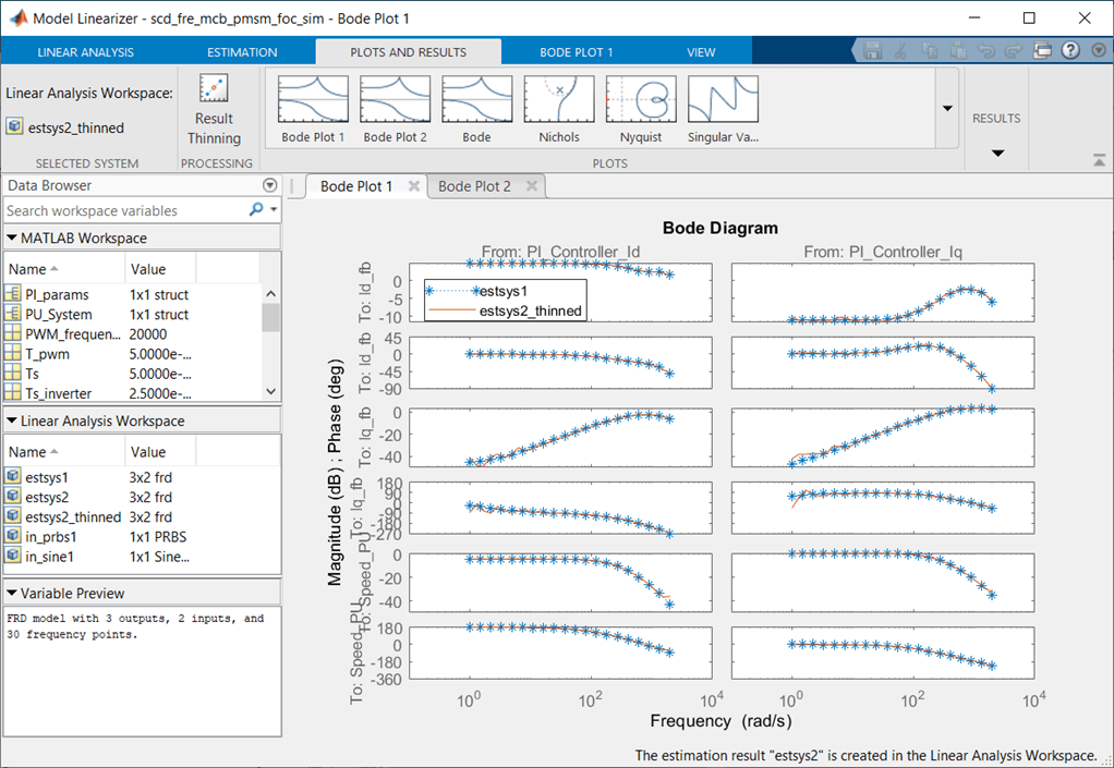
Click OK. The thinned estimated system, estsys2_thinned, appears in the Linear Analysis Workspace. To compare the result with estsys1, click Bode Plot 1.
To find the final simulation time for frequency response estimation by an input signal, select the input signal in the Linear Analysis Workspace and view the simulation time in the Variable Preview area of the Model Linearizer. Alternatively, you can export the input signals to the MATLAB® workspace and use the getSimulationTime function. Load a previously saved session and display the simulation times.
load pmsm_fre_comparison.mat
tfinal_sinestream = in_sine1.getSimulationTime
tfinal_prbs = in_prbs1.getSimulationTime
tfinal_sinestream =

   76.2012


tfinal_prbs =

   13.1071
Both input signals provide similar performances in frequency response estimation. You can use PRBS input signals to obtain accurate frequency response estimation results in a shorter simulation time as compared to estimation with sinestream signals. However, since PRBS estimation results contain a large number of frequency points, you must thin them for accurate parametric estimation.
Estimate Parametric Model from Frequency Response Result
Parametric models, such as transfer function models and state-space models, are widely used in control design workflows. You can estimate a parametric model from the frequency response estimation result.
To estimate a parametric model for the PMSM motor, first export estsys1 or estsys2_thinned to MATLAB workspace, then use tfest or ssest functions from the System Identification Toolbox™ software to estimate a transfer function model or a state-space model, respectively.
Close the model.
close_system(model,0)