Analyze System Dynamics in MATLAB

R2026b

This example shows how to analyze the dynamics of a four-bar linkage system using the MATLAB® classes of Simscape™ Multibody™. The example system is a crank-rocker mechanism that has four links measuring 5 cm, 8 cm, 10 cm, and 12 cm in length.

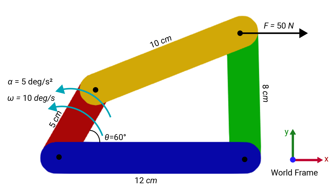
The image shows the initial configuration of the system, where the angle between the crank link and the base link is 60 degrees. The crank link drives the system at an angular velocity of 10 deg/s. An angular acceleration of 5 deg/s² propels the crank link, and a load of 50 N acts on the distal end of the rocker link. This force aligns with the x-axis of the world frame.

Create Four-Bar System

To construct the four-bar multibody system, open the example and use the custom function fourbar with the specified link lengths. For detailed instructions on building a four-bar system in MATLAB, see Model a Multibody System in MATLAB.

import simscape.multibody.* simscape.Value simscape.op.*
[fb,op] = fourBar(simscape.Value(12,"cm"), simscape.Value(10,"cm"), simscape.Value(5,"cm"), simscape.Value(8,"cm"));

The four-bar system operates in the X-Y plane, with gravity acts in the negative y-direction. To specify the gravity, use the simscape.multibody.UniformGravity class.

gravity = UniformGravity(Value([0 -9.80665 0],"m/s^2"));

Before analyzing a multibody system, compile the multibody object.

cfb = compile(fb);

To set the initial joint primitive targets, create an operating point object named jointOP.

jointOP = simscape.op.OperatingPoint;
jointOP("Bottom_Left_Joint/Rz/q") = simscape.op.Target(60,"deg","High");
jointOP("Bottom_Right_Joint/Rz/q") = simscape.op.Target(90,"deg","Low");
jointOP("Bottom_Left_Joint/Rz/w") = simscape.op.Target(10,"deg/s","High");

To verify that the four-bar system meets all the specified targets, compute the state of the system by using the computeState method.

state = computeState(cfb,jointOP)

state = 
  State with properties:

    Status: Valid

The results confirm that the system satisfies all the specified targets.

To visualize the system, use the visualize method. Run this command in your MATLAB Command Window.

visualize(cfb,computeState(cfb,jointOP),"vizFourBar")

Specify Joint Internal Mechanics

In real-life applications, the joints in a mechanical system are not ideal and often experience energy losses. To account for these effects in the revolute joints, specify the spring and damping properties by using the RevolutePrimitiveInternalMechanics class.

To specify spring stiffness and damping coefficient, use the LinearRotationalSpring and LinearRotationalDamper classes:

spring = LinearRotationalSpring(Value(0.5,'N*m/deg'));
damper = LinearRotationalDamper(Value(0.1,'N*m/(deg/s)'));

To set the equilibrium position of the spring, use a simscape.Value object.

eilibriumPosition = Value(90,"deg");

For simplicity, use the same spring and damper properties for all the joints.

im = RevolutePrimitiveInternalMechanics(eilibriumPosition,spring,damper);
Bottom_Left_Joint.InternalMechanics  = im;
Top_Left_Joint.InternalMechanics     = im;
Top_Right_Joint.InternalMechanics    = im;
Bottom_Right_Joint.InternalMechanics = im;

Model Joint Actuation and External Loads

As shown in the system diagram, the crank link drives the system with an angular acceleration of 5 deg/s^2, and a load of 50 N acts on the distal end of the rocker link. To construct the acceleration and load for the system, use the simscape.multibody.JointAccelerationDictionary and simscape.multibody.ExternalForceTorqueDictionary classes.

To pair and store the joint acceleration with the associated joint primitive, use the dict_accel dictionary.

dict_accel = simscape.multibody.JointAccelerationDictionary;
accel_revolute = simscape.multibody.RevolutePrimitiveAcceleration(simscape.Value(5,"deg/s^2"));
dict_accel("Bottom_Left_Joint/Rz") = accel_revolute;

By default, all joint primitives in the system have zero actuation torque. However, the bottom left joint undergoes an angular acceleration. To maintain balance during dynamics computation, specify one joint primitive to automatically compute torque. For example, you can specify the joint primitive between the connector link and the rocker link as automatically computed by using the simscape.multibody.JointActuationDictionary class.

dict_t = simscape.multibody.JointActuationDictionary;
torque = simscape.multibody.RevolutePrimitiveActuationTorque("Computed");
dict_t("Top_Right_Joint/Rz") = torque;

To pair and store the load with the associated frame connector, use the dict_f dictionary. The load aligns with the x-axis of the world frame.

dict_f = simscape.multibody.ExternalForceTorqueDictionary;
force = simscape.multibody.ExternalForce(simscape.Value([50 0 0],"N"),"World");
dict_f("Right_Link/pos_end/f") = force;

Compute Dynamics

To compute the dynamics of the four-bar system using the given state and actuation inputs, use the computeDynamics method.

dynamicsResult = computeDynamics(cfb,state,gravity,dict_accel,dict_t,dict_f);

You can now query the positions, velocities, and accelerations of every joint primitive in the system. For example, to obtain the angular velocity and acceleration of the joint primitive between the base link and the rocker link, use the componentResults method.

vel_bottom_right = componentResults(cfb,"Bottom_Right_Joint",state).Rz.Velocity

vel_bottom_right = 
    0.0723 (rad/s)

accel_bottom_right = componentResults(cfb,"Bottom_Right_Joint",dynamicsResult).Rz.Acceleration

accel_bottom_right = 
    0.0532 (rad/s^2)