Cox Proportional Hazards Model Object
This example shows how to fit and analyze a Cox proportional hazards model using a CoxModel object. Cox proportional hazards models relate to lifetime or failure time data. For background, see What Is Survival Analysis? and Cox Proportional Hazards Model.
Predictors and Stratification Levels
The main assumption in a Cox proportional hazards model is that the hazard rate, meaning the instantaneous failure rate or event rate, is proportional to a base rate at all times . The constant of proportionality depends on the values of predictors, which are called covariates in some literature. The hazard rate for predictors with associated coefficients is
.
This example uses an extension of the Cox proportional hazards model to three stratification levels; see Extension of Cox Proportional Hazards Model. A stratified Cox model has a fixed number of base rates , and the model uses the same predictors and coefficients for all stratification levels.
The proportional hazards assumption implies that a predictor does not depend on time. You might have some time-dependent data to include in the model. To do so in a way that maintains the proportional hazards assumption, create a stratified model. If your data are categorizable, create one stratification per level of your data, and within each stratification, the model uses a different base rate. The base rates can vary in time, so the proportional hazards assumption is maintained. When given values of your time-dependent data as stratification values, the trained model outputs different hazard rates.
Create Data for Fitting
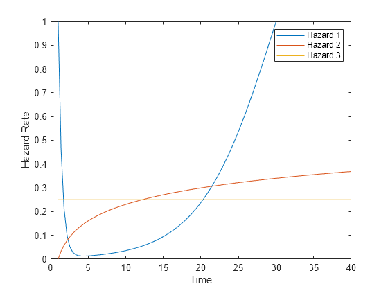
Generate the data for three lifetime models with the following types of hazard rates. These models correspond to three stratification levels.
Bathtub, , whose failure rate is high at the beginning, decreases to a low level, then climbs toward a constant level
Logarithmically increasing:
Constant
The three models share a predictor with three multipliers for the base hazard rates:
11/201/100
In total, the data has nine types of population members, one from each stratification level and one from each predictor level. The functions for creating the bathtub and logarithmic hazard rates are in the Helper Functions section at the end of this example.
Plot the three hazard rates when the predictor value is 1.
t = linspace(1,40);
plot(t,hazard(t),t,log(t)/10,t,1/4*ones(size(t)))
legend('Hazard 1','Hazard 2','Hazard 3','Location','northeast')
ylim([0 1])
xlabel("Time")
ylabel("Hazard Rate")

Create pseudorandom data for the lifetimes associated with the nine models. Create 9000 samples chosen randomly (about 1000 of each type) by inverting the cumulative distributions. (For details, see Inverse transform sampling).
N = 9000;
rng default % For reproducibility
mults = [1;1/20;1/100]; % Three predictors
strata = randi(3,N,1); % Three strata
t1 = zeros(N,1);
a0 = randi(3,N,1); % Predictor
a1 = mults(a0);
v1 = rand(N,1);
for i = 1:N
    switch strata(i)
        case 1 % Bathtub
            t1(i) = zeropt(a1(i),v1(i));
        case 2 % Logarithmic
            t1(i) = zeroptold(a1(i),v1(i));
        case 3 % Constant
            t1(i) = 1 + exprnd(4/a1(i));
    end
end
Place data into a table.
a3 = categorical(a1);
tbldata = table(t1,a3,strata,'VariableNames',["Lifetime" "Predictors" "Strata"]);
Fit Cox Model
Fit a stratified Cox proportional hazards model to the table data.
coxMdl = fitcox(tbldata,'Lifetime ~ Predictors',"Stratification",'Strata');
Plot Survival
Plot the probability of survival as a function of time for a predictor value pred = 1 (or specify any value when you run this example) and the three stratification levels.
pred = 1;
cpred = categorical(pred);
plotSurvival(coxMdl,[cpred;cpred;cpred],[1;2;3])
xlim([1,10/pred + 20])
Even though the hazard rates are proportional for the different predictors, the three survival plots are not proportional because the underlying hazard functions differ.
Analyze Fit
Examine the coefficients of the fitted model.
disp(coxMdl.Coefficients)
                        Beta        SE       zStat     pValue
                       ______    ________    ______    ______

    Predictors_0.05    1.5301    0.031783    48.143      0
    Predictors_1       4.5593    0.052149    87.427      0
Notice that the pValue entries are 0, which means that the listed predictor Beta values are not zero.
View the confidence intervals for the model coefficients at the 0.01 level of significance.
coefci(coxMdl,0.01)
ans = 2×2

    1.4483    1.6120
    4.4249    4.6936
To infer the hazard for the 0.01 level predictor, recall the definition of the Cox model:
.
The fitcox function uses dummy variables with a reference group to handle categorical data. In this case, the function treats the 0.01 level predictor as the reference group, and encodes the predictor as all 0s when fitting the model. If you enter all 0s into the hazard function, you get
is the baseline hazard, which is stored in coxMdl.Hazard. Therefore, to get the hazard for the 0.01 level predictor, you can examine coxMdl.Hazard. Plot the baseline cumulative hazard for the three stratification levels.
figure
hold on
for i = 1:3
    pred3 = find(coxMdl.Hazard(:,3) == i); % Find indices of stratification i
    plot(coxMdl.Hazard(pred3,1),coxMdl.Hazard(pred3,2))
end
xlabel('Time')
ylabel('Cumulative Hazard')
xlim([1 300])
legend('X = 0.01, Stratification 1',...
    'X = 0.01, Stratification 2',...
    'X = 0.01, Stratification 3','Location','northwest')
hold off

The cumulative hazard for the other predictor values is times the baseline cumulative hazard, where is the inferred coefficient.
disp(exp(coxMdl.Coefficients.Beta))
    4.6188
   95.5127
These relative hazard values are close to the theoretical values for the data, which were generated with multipliers 1, 1/20, and 1/100. The baseline value corresponds to the 1/100 multiplier, so the theoretical multipliers are 5 and 100.
View the linhyptest table.
linhyptest(coxMdl)
ans=2×2 table
         Predictor         pValue
    ___________________    ______

    {'Empty Model'    }      0
    {'Predictors_0.05'}      0
Again, the model requires the 1/20 value predictor and the 1 value predictor.
Check whether the data supports the hypothesis that the data is from a Cox proportional hazards model.
supports = coxMdl.ProportionalHazardsPValueGlobal
supports =
0.9730
The null hypothesis for this test is that the data is from a Cox proportional hazards model. To reject this hypothesis, supports must be less than 0.05 or some other small significance level. The statistic indicates support for the hypothesis that the data is consistent with a Cox model.
Examine Hazard Ratios
Calculate the hazard ratio for the predictor values 1, 1/20, and 1/100 compared to a baseline of 0 for the three stratification levels.
hazards = hazardratio(coxMdl,...
    categorical([1;1;1;1/20;1/20;1/20;1/100;1/100;1/100]),...
    [1;2;3;1;2;3;1;2;3],'Baseline',0)
hazards = 9×1

   95.5127
   95.5127
   95.5127
    4.6188
    4.6188
    4.6188
    1.0000
    1.0000
    1.0000
The hazard ratios are near their theoretical values of 100, 5, and 1, as explained in the previous section. The hazard ratios do not depend on the stratification level.
How Well Does the Constant Hazard Stratification Level Match Theory?
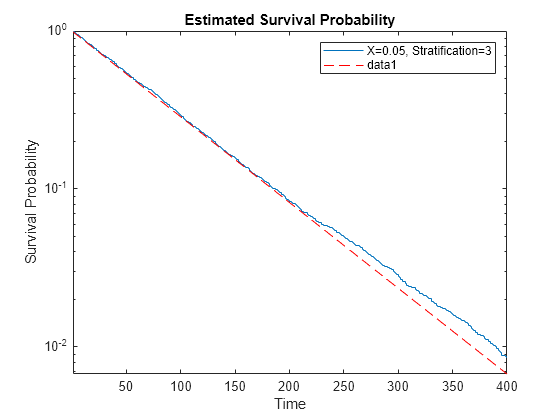
Stratification level 3 has a constant hazard rate of 1/4. Theoretically, a constant hazard rate means an exponential survival function, whose logarithm is a straight line. Plot the survival of level 3 stratification using the predictor value 1/20, which leads to an exponential rate of 1/80.
tt = categorical(1/20);
h = figure;
axes1 = axes('Parent',h);
plotSurvival(coxMdl,axes1,tt,3);
xlim([1 400]);
axes1.YScale = 'log';
hold on
tms = linspace(1,400);
semilogy(tms,exp(-tms/80),'r--')
hold off

The data matches the theoretical line for probabilities well above 1/100.
Reduce Memory Usage by Discarding Residuals
Examine the memory used by the model.
M1 = whos("coxMdl");
disp(M1.bytes)
1231325
Remove the residuals from the model.
coxMdl = discardResiduals(coxMdl);
Examine how the removal affects the memory used by the model.
M2 = whos("coxMdl");
disp(M2.bytes)
437853
disp(M1.bytes/M2.bytes)
2.8122
Removing the residuals decreases the memory usage by nearly a factor of 3.
Helper Functions
This function creates the bathtub hazard rate.
function h = hazard(x)
h = exp(-2*(x - 1)) + (1 + tanh(x/10 - 3));
end
This function creates the integral of the bathtub hazard rate from 1 to x.
function eh = exphazard(x)
eh = 1/2 - exp(-2*(x-1))/2;
eh2 = (10*log(cosh(x/10 - 3)) - 10*log(cosh(1/10 - 3)) + x - 1);
eh = eh + eh2;
end
This function solves for the root of the cumulative hazard rate with multiplier a to level v.
function zz = zeropt(a,v)
zz = fzero(@(x)(1 - exp(-a*exphazard(x)) - v),[1 100*max(1,1/a)]);
end
This function creates the integral of the logarithmic hazard rate with multiplier 1/10 from 1 to x.
function cr = cumrisk(x)
cr = 1/10*(x.*(log(x) - 1) + 1);
end
This function solves for the root of the cumulative hazard rate with multiplier a to level v.
function zz = zeroptold(a,v)
zz = fzero(@(x)(1 - exp(-a*cumrisk(x)) - v),[1 50*max(1,1/a)]);
end