estimateMAP

Class: HamiltonianSampler

Estimate maximum of log probability density

Syntax

xhat = estimateMAP(smp)
[xhat,fitinfo] = estimateMAP(smp)
[xhat,fitinfo] = estimateMAP(___,Name,Value)


Description

xhat = estimateMAP(smp) returns the maximum-a-posteriori (MAP) estimate of the log probability density of the Monte Carlo sampler smp.

[xhat,fitinfo] = estimateMAP(smp) returns additional fitting information in fitinfo.

[xhat,fitinfo] = estimateMAP(___,Name,Value) specifies additional options using one or more name-value pair arguments. Specify name-value pair arguments after all other input arguments.

Input Arguments

smp — Hamiltonian Monte Carlo sampler

HamiltonianSampler object

Hamiltonian Monte Carlo sampler, specified as a HamiltonianSampler object.

estimateMAP estimates the maximum of the log probability density specified in smp.LogPDF.

Use the hmcSampler function to create a sampler.

Name-Value Arguments

Specify optional pairs of arguments as Name1=Value1,...,NameN=ValueN, where Name is the argument name and Value is the corresponding value. Name-value arguments must appear after other arguments, but the order of the pairs does not matter.

Before R2021a, use commas to separate each name and value, and enclose Name in quotes.

Example: 'IterationLimit',100,'StepTolerance',1e-5 estimates the MAP point using an iteration limit of 100 and a step size convergence tolerance of 1e-5.

StartPoint — Initial point to start optimization from

smp.StartPoint (default) | numeric column vector

Initial point to start optimization from, specified as a numeric column vector with the same number of elements as the StartPoint property of the sampler smp.

Example: 'StartPoint',randn(size(smp.StartPoint))

IterationLimit — Maximum number of optimization iterations

1000 (default) | positive integer

Maximum number of optimization iterations, specified as a positive integer.

Example: 'IterationLimit',100

VerbosityLevel — Verbosity level of Command Window output

0 (default) | positive integer

Verbosity level of Command Window output during function maximization, specified as 0 or a positive integer.

• With the value set to 0, estimateMAP displays no details on the optimization.

• With the value set to a positive integer, estimateMAP displays convergence information at each iteration.

Convergence Information

Heading	Meaning
FUN VALUE	Objective function value.
NORM GRAD	Norm of the gradient of the objective function.
NORM STEP	Norm of the iterative step, meaning the distance between the previous point and the current point.
CURV	OK means the weak Wolfe condition is satisfied. This condition is a combination of sufficient decrease of the objective function and a curvature condition.
GAMMA	Inner product of the step times the gradient difference, divided by the inner product of the gradient difference with itself. The gradient difference is the gradient at the current point minus the gradient at the previous point. Gives diagnostic information on the objective function curvature.
ALPHA	Step direction multiplier, which differs from 1 when the algorithm performed a line search.
ACCEPT	YES means the algorithm found an acceptable step to take.

Example: 'VerbosityLevel',1

GradientTolerance — Relative gradient convergence tolerance

1e-6 (default) | positive scalar

Relative gradient convergence tolerance, specified as a positive scalar.

Let tau = max(1,min(abs(f),infnormg0)), where f is the current objective function value and infnormg0 is the initial gradient norm. If the norm of the objective function gradient is smaller than tau times the 'GradientTolerance' value, then the maximization is considered to have converged to a local optimum.

Example: 'GradientTolerance',1e-4

StepTolerance — Step size convergence tolerance

1e-6 (default) | positive scalar

Step size convergence tolerance, specified as a positive scalar.

If the proposed step size is smaller than the 'StepTolerance' value, then the maximization is considered to have converged to a local optimum.

Example: 'StepTolerance',1e-5

Output Arguments

xhat — MAP point estimate

numeric vector

MAP point estimate, returned as a numeric vector of the same size as smp.StartPoint.

fitinfo — Fitting information

structure

Fitting information for the MAP computation, returned as a structure with these fields:

Field	Description
Iteration	Iteration indices from 0 through the final iteration.
Objective	Negative log probability density at each iteration. The MAP point is computed by minimizing the negative log probability density. You can check that the final values are all similar, indicating that the function optimization has converged to a local optimum.
Gradient	Gradient of the negative log probability density at the final iteration.

Data Types: struct

Examples

Estimate MAP Point of HMC Sampler

Create a Hamiltonian Monte Carlo sampler for a normal distribution and estimate the maximum-a-posteriori (MAP) point of the log probability density.

First, save a function normalDistGrad on the MATLAB® path that returns the multivariate normal log probability density and its gradient (normalDistGrad is defined at the end of this example). Then, call the function with arguments to define the logpdf input argument to the hmcSampler function.

means = [1;-1];
standevs = [1;0.3];
logpdf = @(theta)normalDistGrad(theta,means,standevs);

Choose a starting point and create the HMC sampler.

startpoint = zeros(2,1);
smp = hmcSampler(logpdf,startpoint);

Estimate the MAP point (the point where the probability density has its maximum). Show more information during optimization by setting the 'VerbosityLevel' value to 1.

[xhat,fitinfo] = estimateMAP(smp,'VerbosityLevel',1);

 o Solver = LBFGS, HessianHistorySize = 15, LineSearchMethod = weakwolfe

|====================================================================================================|
|   ITER   |   FUN VALUE   |  NORM GRAD  |  NORM STEP  |  CURV  |    GAMMA    |    ALPHA    | ACCEPT |
|====================================================================================================|
|        0 |  6.689460e+00 |   1.111e+01 |   0.000e+00 |        |   9.000e-03 |   0.000e+00 |   YES  |
|        1 |  4.671622e+00 |   8.889e+00 |   2.008e-01 |    OK  |   9.006e-02 |   2.000e+00 |   YES  |
|        2 |  9.759850e-01 |   8.268e-01 |   8.215e-01 |    OK  |   9.027e-02 |   1.000e+00 |   YES  |
|        3 |  9.158025e-01 |   7.496e-01 |   7.748e-02 |    OK  |   5.910e-01 |   1.000e+00 |   YES  |
|        4 |  6.339508e-01 |   3.104e-02 |   7.472e-01 |    OK  |   9.796e-01 |   1.000e+00 |   YES  |
|        5 |  6.339043e-01 |   3.668e-05 |   3.762e-03 |    OK  |   9.599e-02 |   1.000e+00 |   YES  |
|        6 |  6.339043e-01 |   2.488e-08 |   3.333e-06 |    OK  |   9.015e-02 |   1.000e+00 |   YES  |

         Infinity norm of the final gradient = 2.488e-08
              Two norm of the final step     = 3.333e-06, TolX   = 1.000e-06
Relative infinity norm of the final gradient = 2.488e-08, TolFun = 1.000e-06
EXIT: Local minimum found.

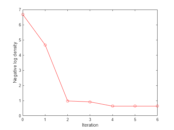
To further check that the optimization has converged to a local minimum, plot the fitinfo.Objective field. This field contains the values of the negative log density at each iteration of the function optimization. The final values are all very similar, so the optimization has converged.

fitinfo

fitinfo = struct with fields:
    Iteration: [7×1 double]
    Objective: [7×1 double]
     Gradient: [2×1 double]

plot(fitinfo.Iteration,fitinfo.Objective,'ro-');
xlabel('Iteration');
ylabel('Negative log density');

Display the MAP estimate. It is indeed equal to the means variable, which is the exact maximum.

xhat

xhat = 2×1

    1.0000
   -1.0000

means

means = 2×1

     1
    -1

The normalDistGrad function returns the logarithm of the multivariate normal probability density with means in Mu and standard deviations in Sigma, specified as scalars or columns vectors the same length as startpoint. The second output argument is the corresponding gradient.

function [lpdf,glpdf] = normalDistGrad(X,Mu,Sigma)
Z = (X - Mu)./Sigma;
lpdf = sum(-log(Sigma) - .5*log(2*pi) - .5*(Z.^2));
glpdf = -Z./Sigma;
end

Tips

• First create a Hamiltonian Monte Carlo sampler using the hmcSampler function, and then use estimateMAP to estimate the MAP point.

• After creating an HMC sampler, you can tune the sampler, draw samples, and check convergence diagnostics using the other methods of the HamiltonianSampler class. Using the MAP estimate as a starting point in the tuneSampler and drawSamles methods can lead to more efficient tuning and sampling. For an example of this workflow, see Bayesian Linear Regression Using Hamiltonian Monte Carlo.

Algorithms

• estimateMAP uses a limited memory Broyden-Fletcher-Goldfarb-Shanno (LBFGS) quasi-Newton optimizer to search for the maximum of the log probability density. See Nocedal and Wright [1].

References

[1] Nocedal, J. and S. J. Wright. Numerical Optimization, Second Edition. Springer Series in Operations Research, Springer Verlag, 2006.

Version History

Introduced in R2017a