Introduction to Fairness in Binary Classification

The functions fairnessMetrics, fairnessWeights, disparateImpactRemover, and fairnessThresholder in Statistics and Machine Learning Toolbox™ allow you to detect and mitigate societal bias in binary classification. First, use fairnessMetrics to evaluate the fairness of a data set or classification model with bias and group metrics. Then, use fairnessWeights to reweight observations, disparateImpactRemover to remove the disparate impact of a sensitive attribute, or fairnessThresholder to optimize the classification threshold.

• fairnessMetrics — The fairnessMetrics function computes fairness metrics (bias metrics and group metrics) for a data set or binary classification model with respect to sensitive attributes. The data-level evaluation examines binary, true labels of the data. The model-level evaluation examines the predicted labels returned by one or more binary classification models, using both true labels and predicted labels. You can use the metrics to determine if your data or models contain bias toward a group within each sensitive attribute.

• fairnessWeights — The fairnessWeights function computes fairness weights with respect to a sensitive attribute and the response variable. For every combination of a group in the sensitive attribute and a class label in the response variable, the software computes a weight value. The function then assigns each observation its corresponding weight. The returned weights introduce fairness across the sensitive attribute groups. Pass the weights to an appropriate training function, such as fitcsvm, using the Weights name-value argument.

• disparateImpactRemover — The disparateImpactRemover function tries to remove the disparate impact of a sensitive attribute on model predictions by using the sensitive attribute to transform the continuous predictors in the data set. The function returns the transformed data set and a disparateImpactRemover object that contains the transformation. Pass the transformed data set to an appropriate training function, such as fitcsvm, and pass the object to the transform object function to apply the transformation to a new data set, such as a test data set.

• fairnessThresholder — The fairnessThresholder function searches for an optimal score threshold to maximize accuracy while satisfying fairness bounds. For observations in the critical region below the optimal threshold, the function adjusts the labels so that the fairness constraints hold for the reference and nonreference groups in the sensitive attribute. After you create a fairnessThresholder object, you can use the predict and loss object functions on new data to predict fairness labels and calculate the classification loss, respectively.

Reduce Statistical Parity Difference Using Fairness Weights

Train a neural network model, and compute the statistical parity difference (SPD) for each group in the sensitive attribute. To reduce the SPD values, compute fairness weights, and retrain the neural network model.

Read the sample file CreditRating_Historical.dat into a table. The predictor data consists of financial ratios and industry sector information for a list of corporate customers. The response variable consists of credit ratings assigned by a rating agency.

creditrating = readtable("CreditRating_Historical.dat");

Because each value in the ID variable is a unique customer ID—that is, length(unique(creditrating.ID)) is equal to the number of observations in creditrating—the ID variable is a poor predictor. Remove the ID variable from the table, and convert the Industry variable to a categorical variable.

creditrating.ID = [];
creditrating.Industry = categorical(creditrating.Industry);

In the Rating response variable, combine the AAA, AA, A, and BBB ratings into a category of "good" ratings, and the BB, B, and CCC ratings into a category of "poor" ratings.

Rating = categorical(creditrating.Rating);
Rating = mergecats(Rating,["AAA","AA","A","BBB"],"good");
Rating = mergecats(Rating,["BB","B","CCC"],"poor");
creditrating.Rating = Rating;

Train a neural network model on the creditrating data. For better results, standardize the predictors before fitting the model. Use the trained model to predict labels for the training data set.

rng("default") % For reproducibility
netMdl = fitcnet(creditrating,"Rating",Standardize=true);
netPredictions = predict(netMdl,creditrating);

Compute fairness metrics with respect to the Industry sensitive attribute by using the model predictions. In particular, find the statistical parity difference (SPD) for each group in Industry.

netEvaluator = fairnessMetrics(creditrating,"Rating", ...
    SensitiveAttributeNames="Industry",Predictions=netPredictions);
report(netEvaluator,BiasMetrics="StatisticalParityDifference")

ans=12×4 table
    ModelNames    SensitiveAttributeNames    Groups    StatisticalParityDifference
    __________    _______________________    ______    ___________________________

      Model1             Industry              1                 0.065724         
      Model1             Industry              2                 0.078449         
      Model1             Industry              3                        0         
      Model1             Industry              4                 0.097937         
      Model1             Industry              5                  0.05251         
      Model1             Industry              6               -0.0061672         
      Model1             Industry              7                 0.030037         
      Model1             Industry              8                 0.087863         
      Model1             Industry              9                  0.16367         
      Model1             Industry              10                 0.15076         
      Model1             Industry              11                0.019402         
      Model1             Industry              12                0.032187         

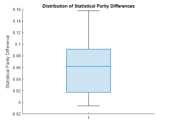
To better understand the distribution of SPD values, plot the values using a box plot.

spdValues = netEvaluator.BiasMetrics.StatisticalParityDifference;
boxchart(spdValues)
ylabel("Statistical Parity Difference")
title("Distribution of Statistical Parity Differences")

The median SPD value is around 0.06, which is higher than the value 0 of a fair model.

Compute fairness weights, and refit a neural network model using the weights. As before, standardize the predictors. Then, predict labels for the training data by using the new model.

weights = fairnessWeights(creditrating,"Industry","Rating");

rng("default") % For reproducibility
newNetMdl = fitcnet(creditrating,"Rating",Weights=weights, ...
    Standardize=true);
newNetPredictions = predict(newNetMdl,creditrating);

Compute the new SPD values.

newNetEvaluator = fairnessMetrics(creditrating,"Rating", ...
    SensitiveAttributeNames="Industry",Predictions=newNetPredictions);
report(newNetEvaluator,BiasMetrics="StatisticalParityDifference")

ans=12×4 table
    ModelNames    SensitiveAttributeNames    Groups    StatisticalParityDifference
    __________    _______________________    ______    ___________________________

      Model1             Industry              1                 0.051528         
      Model1             Industry              2                 0.070411         
      Model1             Industry              3                        0         
      Model1             Industry              4                  0.06844         
      Model1             Industry              5                 0.029635         
      Model1             Industry              6               -0.0051521         
      Model1             Industry              7                 0.016443         
      Model1             Industry              8                 0.070997         
      Model1             Industry              9                  0.11324         
      Model1             Industry              10                 0.11538         
      Model1             Industry              11                0.026125         
      Model1             Industry              12               0.0090789         

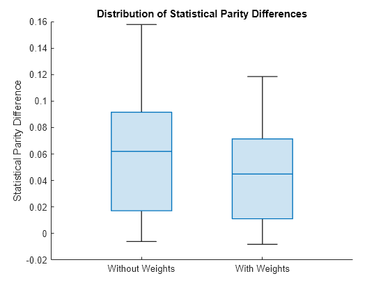
Display the two distributions of SPD values. The left box plot shows the SPD values computed using the original model. The right box plot shows the SPD values computed using the new model trained with fairness weights.

spdValuesUpdated = newNetEvaluator.BiasMetrics.StatisticalParityDifference;
boxchart([spdValues spdValuesUpdated])
xticklabels(["Without Weights","With Weights"])
ylabel("Statistical Parity Difference")
title("Distribution of Statistical Parity Differences")

The new SPD values have a median around 0.04, which is closer to 0 than the previous median of 0.06. The maximum value of the new SPD values, which is around 0.11, is also closer to 0 than the previous maximum value, which is around 0.16.

Reduce Disparate Impact of Predictions

Train a binary classifier, classify test data using the model, and compute the disparate impact for each group in the sensitive attribute. To reduce the disparate impact values, use disparateImpactRemover, and then retrain the binary classifier. Transform the test data set, reclassify the observations, and compute the disparate impact values.

Load the sample data census1994, which contains the training data adultdata and the test data adulttest. The data sets consist of demographic information from the US Census Bureau that can be used to predict whether an individual makes over $50,000 per year. Preview the first few rows of the training data set.

load census1994
head(adultdata)

    age       workClass          fnlwgt      education    education_num       marital_status           occupation        relationship     race      sex      capital_gain    capital_loss    hours_per_week    native_country    salary
    ___    ________________    __________    _________    _____________    _____________________    _________________    _____________    _____    ______    ____________    ____________    ______________    ______________    ______

    39     State-gov                77516    Bachelors         13          Never-married            Adm-clerical         Not-in-family    White    Male          2174             0                40          United-States     <=50K 
    50     Self-emp-not-inc         83311    Bachelors         13          Married-civ-spouse       Exec-managerial      Husband          White    Male             0             0                13          United-States     <=50K 
    38     Private             2.1565e+05    HS-grad            9          Divorced                 Handlers-cleaners    Not-in-family    White    Male             0             0                40          United-States     <=50K 
    53     Private             2.3472e+05    11th               7          Married-civ-spouse       Handlers-cleaners    Husband          Black    Male             0             0                40          United-States     <=50K 
    28     Private             3.3841e+05    Bachelors         13          Married-civ-spouse       Prof-specialty       Wife             Black    Female           0             0                40          Cuba              <=50K 
    37     Private             2.8458e+05    Masters           14          Married-civ-spouse       Exec-managerial      Wife             White    Female           0             0                40          United-States     <=50K 
    49     Private             1.6019e+05    9th                5          Married-spouse-absent    Other-service        Not-in-family    Black    Female           0             0                16          Jamaica           <=50K 
    52     Self-emp-not-inc    2.0964e+05    HS-grad            9          Married-civ-spouse       Exec-managerial      Husband          White    Male             0             0                45          United-States     >50K  

Each row contains the demographic information for one adult. The last column salary shows whether a person has a salary less than or equal to $50,000 per year or greater than $50,000 per year.

Remove observations from adultdata and adulttest that contain missing values.

adultdata = rmmissing(adultdata);
adulttest = rmmissing(adulttest);

Specify the continuous numeric predictors to use for model training.

predictors = ["age","education_num","capital_gain","capital_loss", ...
    "hours_per_week"];

Train an ensemble classifier using the training set adultdata. Specify salary as the response variable and fnlwgt as the observation weights. Because the training set is imbalanced, use the RUSBoost algorithm. After training the model, predict the salary (class label) of the observations in the test set adulttest.

rng("default") % For reproducibility
mdl = fitcensemble(adultdata,"salary",Weights="fnlwgt", ...
    PredictorNames=predictors,Method="RUSBoost");
labels = predict(mdl,adulttest);

Transform the training set predictors by using the race sensitive attribute.

[remover,newadultdata] = disparateImpactRemover(adultdata, ...
    "race",PredictorNames=predictors);
remover

remover = 
  disparateImpactRemover with properties:

        RepairFraction: 1
        PredictorNames: {'age'  'education_num'  'capital_gain'  'capital_loss'  'hours_per_week'}
    SensitiveAttribute: 'race'

remover is a disparateImpactRemover object, which contains the transformation of the remover.PredictorNames predictors with respect to the remover.SensitiveAttribute variable.

Apply the same transformation stored in remover to the test set predictors. Note: You must transform both the training and test data sets before passing them to a classifier.

newadulttest = transform(remover,adulttest, ...
    PredictorNames=predictors);

Train the same type of ensemble classifier as mdl, but use the transformed predictor data. As before, predict the salary (class label) of the observations in the test set adulttest.

rng("default") % For reproducibility
newMdl = fitcensemble(newadultdata,"salary",Weights="fnlwgt", ...
    PredictorNames=predictors,Method="RUSBoost");
newLabels = predict(newMdl,newadulttest);

Compare the disparate impact values for the predictions made by the original model (mdl) and the predictions made by the model trained with the transformed data (newMdl). For each group in the sensitive attribute, the disparate impact value is the proportion of predictions in that group with a positive class value ($$p_{g+}$$) divided by the proportion of predictions in the reference group with a positive class value ($$p_{r+}$$). An ideal classifier makes predictions where, for each group, $$p_{g+}$$ is close to $$p_{r+}$$ (that is, where the disparate impact value is close to 1).

Compute the disparate impact values for the mdl predictions and the newMdl predictions by using fairnessMetrics. Include the observation weights. You can use the report object function to display bias metrics, such as disparate impact, that are stored in the evaluator object.

evaluator = fairnessMetrics(adulttest,"salary", ...
    SensitiveAttributeNames="race",Predictions=[labels,newLabels], ...
    Weights="fnlwgt",ModelNames=["Original Model","New Model"]);
evaluator.PositiveClass

ans = categorical
     >50K 

evaluator.ReferenceGroup

ans = 
'White'

report(evaluator,BiasMetrics="DisparateImpact")

ans=5×5 table
        Metrics        SensitiveAttributeNames          Groups          Original Model    New Model
    _______________    _______________________    __________________    ______________    _________

    DisparateImpact             race              Amer-Indian-Eskimo       0.41702         0.92804 
    DisparateImpact             race              Asian-Pac-Islander         1.719          0.9697 
    DisparateImpact             race              Black                    0.60571         0.66629 
    DisparateImpact             race              Other                    0.66958         0.86039 
    DisparateImpact             race              White                          1               1 

For the mdl predictions, several of the disparate impact values are below the industry standard of 0.8, and one value is above 1.25. These values indicate bias in the predictions with respect to the positive class >50K and the sensitive attribute race.

The disparate impact values for the newMdl predictions are closer to 1 than the disparate impact values for the mdl predictions. One value is still below 0.8.

Visually compare the disparate impact values by using the bar graph returned by the plot object function.

plot(evaluator,"DisparateImpact")

The disparateImpactRemover function seems to have improved the model predictions on the test set with respect to the disparate impact metric.

Check whether the transformed predictors negatively affect the accuracy of the model predictions. Compute the accuracy of the test set predictions for the two models mdl and newMdl.

accuracy = 1-loss(mdl,adulttest,"salary")

accuracy = 
0.8024

newAccuracy = 1-loss(newMdl,newadulttest,"salary")

newAccuracy = 
0.7955

The model trained using the transformed predictors (newMdl) achieves similar test set accuracy compared to the model trained with the original predictors (mdl).