Main Content

kstest

One-sample Kolmogorov-Smirnov test

Description

example

h = kstest(x) returns a test decision for the null hypothesis that the data in vector x comes from a standard normal distribution, against the alternative that it does not come from such a distribution, using the one-sample Kolmogorov-Smirnov test. The result h is 1 if the test rejects the null hypothesis at the 5% significance level, or 0 otherwise.

example

h = kstest(x,Name,Value) returns a test decision for the one-sample Kolmogorov-Smirnov test with additional options specified by one or more name-value pair arguments. For example, you can test for a distribution other than standard normal, change the significance level, or conduct a one-sided test.

example

[h,p] = kstest(___) also returns the p-value p of the hypothesis test, using any of the input arguments from the previous syntaxes.

example

[h,p,ksstat,cv] = kstest(___) also returns the value of the test statistic ksstat and the approximate critical value cv of the test.

Examples

collapse all

Perform the one-sample Kolmogorov-Smirnov test by using kstest. Confirm the test decision by visually comparing the empirical cumulative distribution function (cdf) to the standard normal cdf.

Load the examgrades data set. Create a vector containing the first column of the exam grade data.

load examgrades
test1 = grades(:,1);

Test the null hypothesis that the data comes from a normal distribution with a mean of 75 and a standard deviation of 10. Use these parameters to center and scale each element of the data vector, because kstest tests for a standard normal distribution by default.

x = (test1-75)/10;
h = kstest(x)
h = logical
   0

The returned value of h = 0 indicates that kstest fails to reject the null hypothesis at the default 5% significance level.

Plot the empirical cdf and the standard normal cdf for a visual comparison.

cdfplot(x)
hold on
x_values = linspace(min(x),max(x));
plot(x_values,normcdf(x_values,0,1),'r-')
legend('Empirical CDF','Standard Normal CDF','Location','best')

Figure contains an axes object. The axes object with title Empirical CDF, xlabel x, ylabel F(x) contains 2 objects of type line. These objects represent Empirical CDF, Standard Normal CDF.

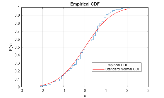
The figure shows the similarity between the empirical cdf of the centered and scaled data vector and the cdf of the standard normal distribution.

Load the sample data. Create a vector containing the first column of the students’ exam grades data.

load examgrades;
x = grades(:,1);

Specify the hypothesized distribution as a two-column matrix. Column 1 contains the data vector x. Column 2 contains cdf values evaluated at each value in x for a hypothesized Student’s t distribution with a location parameter of 75, a scale parameter of 10, and one degree of freedom.

test_cdf = [x,cdf('tlocationscale',x,75,10,1)];

Test if the data are from the hypothesized distribution.

h = kstest(x,'CDF',test_cdf)
h = logical
   1

The returned value of h = 1 indicates that kstest rejects the null hypothesis at the default 5% significance level.

Load the sample data. Create a vector containing the first column of the students’ exam grades data.

load examgrades;
x = grades(:,1);

Create a probability distribution object to test if the data comes from a Student’s t distribution with a location parameter of 75, a scale parameter of 10, and one degree of freedom.

test_cdf = makedist('tlocationscale','mu',75,'sigma',10,'nu',1);

Test the null hypothesis that the data comes from the hypothesized distribution.

h = kstest(x,'CDF',test_cdf)
h = logical
   1

The returned value of h = 1 indicates that kstest rejects the null hypothesis at the default 5% significance level.

Load the sample data. Create a vector containing the first column of the students’ exam grades.

load examgrades;
x = grades(:,1);

Create a probability distribution object to test if the data comes from a Student’s t distribution with a location parameter of 75, a scale parameter of 10, and one degree of freedom.

test_cdf = makedist('tlocationscale','mu',75,'sigma',10,'nu',1);

Test the null hypothesis that data comes from the hypothesized distribution at the 1% significance level.

[h,p] = kstest(x,'CDF',test_cdf,'Alpha',0.01)
h = logical
   1

p = 0.0021

The returned value of h = 1 indicates that kstest rejects the null hypothesis at the 1% significance level.

Load the sample data. Create a vector containing the third column of the stock return data matrix.

load stockreturns;
x = stocks(:,3);

Test the null hypothesis that the data comes from a standard normal distribution, against the alternative hypothesis that the population cdf of the data is larger than the standard normal cdf.

[h,p,k,c] = kstest(x,'Tail','larger')
h = logical
   1

p = 5.0854e-05
k = 0.2197
c = 0.1207

The returned value of h = 1 indicates that kstest rejects the null hypothesis in favor of the alternative hypothesis at the default 5% significance level.

Plot the empirical cdf and the standard normal cdf for a visual comparison.

[f,x_values] = ecdf(x);
J = plot(x_values,f);
hold on;
K = plot(x_values,normcdf(x_values),'r--');
set(J,'LineWidth',2);
set(K,'LineWidth',2);
legend([J K],'Empirical CDF','Standard Normal CDF','Location','SE');

Figure contains an axes object. The axes object contains 2 objects of type line. These objects represent Empirical CDF, Standard Normal CDF.

The plot shows the difference between the empirical cdf of the data vector x and the cdf of the standard normal distribution.

Input Arguments

collapse all

Sample data, specified as a vector.

Data Types: single | double

Name-Value Arguments

Specify optional pairs of arguments as Name1=Value1,...,NameN=ValueN, where Name is the argument name and Value is the corresponding value. Name-value arguments must appear after other arguments, but the order of the pairs does not matter.

Before R2021a, use commas to separate each name and value, and enclose Name in quotes.

Example: 'Tail','larger','Alpha',0.01 specifies a test using the alternative hypothesis that the cdf of the population from which the sample data is drawn is greater than the cdf of the hypothesized distribution, conducted at the 1% significance level.

Significance level of the hypothesis test, specified as the comma-separated pair consisting of 'Alpha' and a scalar value in the range (0,1).

Example: 'Alpha',0.01

Data Types: single | double

cdf of hypothesized continuous distribution, specified the comma-separated pair consisting of 'CDF' and either a two-column matrix or a continuous probability distribution object. When CDF is a matrix, column 1 contains a set of possible x values, and column 2 contains the corresponding hypothesized cumulative distribution function values G(x). The calculation is most efficient if CDF is specified such that column 1 contains the values in the data vector x. If there are values in x not found in column 1 of CDF, kstest approximates G(x) by interpolation. All values in x must lie in the interval between the smallest and largest values in the first column of CDF. By default, kstest tests for a standard normal distribution.

The one-sample Kolmogorov-Smirnov test is only valid for continuous cumulative distribution functions, and requires CDF to be predetermined. The result is not accurate if CDF is estimated from the data. To test x against the normal, lognormal, extreme value, Weibull, or exponential distribution without specifying distribution parameters, use lillietest instead.

Data Types: single | double

Type of alternative hypothesis to evaluate, specified as the comma-separated pair consisting of 'Tail' and one of the following.

'unequal'Test the alternative hypothesis that the cdf of the population from which x is drawn is not equal to the cdf of the hypothesized distribution.
'larger'Test the alternative hypothesis that the cdf of the population from which x is drawn is greater than the cdf of the hypothesized distribution.
'smaller'Test the alternative hypothesis that the cdf of the population from which x is drawn is less than the cdf of the hypothesized distribution.

If the values in the data vector x tend to be larger than expected from the hypothesized distribution, the empirical distribution function of x tends to be smaller, and vice versa.

Example: 'Tail','larger'

Output Arguments

collapse all

Hypothesis test result, returned as a logical value.

  • If h = 1, this indicates the rejection of the null hypothesis at the Alpha significance level.

  • If h = 0, this indicates a failure to reject the null hypothesis at the Alpha significance level.

p-value of the test, returned as a scalar value in the range [0,1]. p is the probability of observing a test statistic as extreme as, or more extreme than, the observed value under the null hypothesis. Small values of p cast doubt on the validity of the null hypothesis.

Test statistic of the hypothesis test, returned as a nonnegative scalar value.

Critical value, returned as a nonnegative scalar value.

More About

collapse all

One-Sample Kolmogorov-Smirnov Test

The one-sample Kolmogorov-Smirnov test is a nonparametric test of the null hypothesis that the population cdf of the data is equal to the hypothesized cdf.

The two-sided test for “unequal” cdf functions tests the null hypothesis against the alternative that the population cdf of the data is not equal to the hypothesized cdf. The test statistic is the maximum absolute difference between the empirical cdf calculated from x and the hypothesized cdf:

D*=maxx(|F^(x)G(x)|),

where F^(x) is the empirical cdf and G(x) is the cdf of the hypothesized distribution.

The one-sided test for a “larger” cdf function tests the null hypothesis against the alternative that the population cdf of the data is greater than the hypothesized cdf. The test statistic is the maximum amount by which the empirical cdf calculated from x exceeds the hypothesized cdf:

D*=maxx(F^(x)G(x)).

The one-sided test for a “smaller” cdf function tests the null hypothesis against the alternative that the population cdf of the data is less than the hypothesized cdf. The test statistic is the maximum amount by which the hypothesized cdf exceeds the empirical cdf calculated from x:

D*=maxx(G(x)F^(x)).

kstest computes the critical value cv using an approximate formula or by interpolation in a table. The formula and table cover the range 0.01alpha0.2 for two-sided tests and 0.005alpha0.1 for one-sided tests. cv is returned as NaN if alpha is outside this range.

Algorithms

kstest decides to reject the null hypothesis by comparing the p-value p with the significance level Alpha, not by comparing the test statistic ksstat with the critical value cv. Since cv is approximate, comparing ksstat with cv occasionally leads to a different conclusion than comparing p with Alpha.

References

[1] Massey, F. J. “The Kolmogorov-Smirnov Test for Goodness of Fit.” Journal of the American Statistical Association. Vol. 46, No. 253, 1951, pp. 68–78.

[2] Miller, L. H. “Table of Percentage Points of Kolmogorov Statistics.” Journal of the American Statistical Association. Vol. 51, No. 273, 1956, pp. 111–121.

[3] Marsaglia, G., W. Tsang, and J. Wang. “Evaluating Kolmogorov’s Distribution.” Journal of Statistical Software. Vol. 8, Issue 18, 2003.

Version History

Introduced before R2006a