Detect Outliers Using Quantile Regression

This example shows how to detect outliers using quantile random forest. Quantile random forest can detect outliers with respect to the conditional distribution of $$Y$$ given $$X$$. However, this method cannot detect outliers in the predictor data. For outlier detection in the predictor data using a bag of decision trees, see the OutlierMeasure property of a TreeBagger model.

An outlier is an observation that is located far enough from most of the other observations in a data set and can be considered anomalous. Causes of outlying observations include inherent variability or measurement error. Outliers significantly affect estimates and inference, so it is important to detect them and decide whether to remove them or consider a robust analysis.

To demonstrate outlier detection, this example:

1. Generates data from a nonlinear model with heteroscedasticity and simulates a few outliers.

2. Grows a quantile random forest of regression trees.

3. Estimates conditional quartiles ($$Q_1$$, $$Q_2$$, and $$Q_3$$) and the interquartile range ($$IQR$$) within the ranges of the predictor variables.

4. Compares the observations to the fences, which are the quantities $$F_1=Q_1-1.5IQR$$ and $$F_2=Q_3+1.5IQR$$. Any observation that is less than $$F_1$$ or greater than $$F_2$$ is an outlier.

Generate Data

Generate 500 observations from the model

$$y_t=10+3t+t\sin (2t)+{\epsilon }_t.$$

$$t$$ is uniformly distributed between 0 and $$4\pi$$, and $${\epsilon }_t\sim N(0,t+0.01)$$. Store the data in a table.

n = 500;
rng('default'); % For reproducibility
t = randsample(linspace(0,4*pi,1e6),n,true)';
epsilon = randn(n,1).*sqrt((t+0.01));
y = 10 + 3*t + t.*sin(2*t) + epsilon;

Tbl = table(t,y);

Move five observations in a random vertical direction by 90% of the value of the response.

numOut = 5;
[~,idx] = datasample(Tbl,numOut);
Tbl.y(idx) = Tbl.y(idx) + randsample([-1 1],numOut,true)'.*(0.9*Tbl.y(idx));

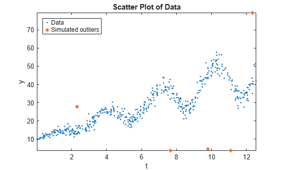
Draw a scatter plot of the data and identify the outliers.

figure;
plot(Tbl.t,Tbl.y,'.');
hold on
plot(Tbl.t(idx),Tbl.y(idx),'*');
axis tight;
ylabel('y');
xlabel('t');
title('Scatter Plot of Data');
legend('Data','Simulated outliers','Location','NorthWest');

Grow Quantile Random Forest

Grow a bag of 200 regression trees using TreeBagger.

Mdl = TreeBagger(200,Tbl,'y','Method','regression');

Mdl is a TreeBagger ensemble.

Predict Conditional Quartiles and Interquartile Ranges

Using quantile regression, estimate the conditional quartiles of 50 equally spaced values within the range of t.

tau = [0.25 0.5 0.75];
predT = linspace(0,4*pi,50)';
quartiles = quantilePredict(Mdl,predT,'Quantile',tau);

quartiles is a 500-by-3 matrix of conditional quartiles. Rows correspond to the observations in t, and columns correspond to the probabilities in tau.

On the scatter plot of the data, plot the conditional mean and median responses.

meanY = predict(Mdl,predT);

plot(predT,[quartiles(:,2) meanY],'LineWidth',2);
legend('Data','Simulated outliers','Median response','Mean response',...
    'Location','NorthWest');
hold off;

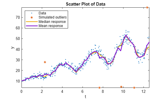
Although the conditional mean and median curves are close, the simulated outliers can affect the mean curve.

Compute the conditional $$IQR$$, $$F_1$$, and $$F_2$$.

iqr = quartiles(:,3) - quartiles(:,1);
k = 1.5;
f1 = quartiles(:,1) - k*iqr;
f2 = quartiles(:,3) + k*iqr;

k = 1.5 means that all observations less than f1 or greater than f2 are considered outliers, but this threshold does not disambiguate from extreme outliers. A k of 3 identifies extreme outliers.

Compare Observations to Fences

Plot the observations and the fences.

figure;
plot(Tbl.t,Tbl.y,'.');
hold on
plot(Tbl.t(idx),Tbl.y(idx),'*');
plot(predT,[f1 f2]);
legend('Data','Simulated outliers','F_1','F_2','Location','NorthWest');
axis tight
title('Outlier Detection Using Quantile Regression')
hold off

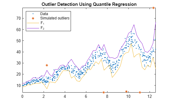
All simulated outliers fall outside $$[F_1,F_2]$$, and some observations are outside this interval as well.