Visualize Decision Surfaces of Different Classifiers

This example shows how to plot the decision surface of different classification algorithms.

Load Fisher's iris data set.

load fisheriris
X = meas(:,1:2);
y = categorical(species);
labels = categories(y);

X is a numeric matrix that contains two petal measurements for 150 irises. Y is a cell array of character vectors that contains the corresponding iris species.

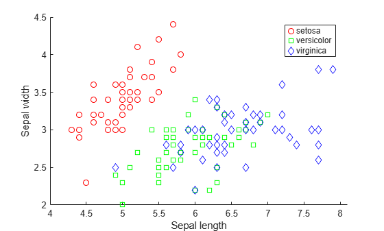
Visualize the data using a scatter plot. Group the variables by iris species.

gscatter(X(:,1),X(:,2),species,'rgb','osd');
xlabel('Sepal length');
ylabel('Sepal width');

Train four different classifiers and store the models in a cell array.

classifier_name = {'Naive Bayes','Discriminant Analysis','Classification Tree','Nearest Neighbor'};

Train a naive Bayes model.

classifier{1} = fitcnb(X,y);

Train a discriminant analysis classifier.

classifier{2} = fitcdiscr(X,y);

Train a classification decision tree.

classifier{3} = fitctree(X,y);

Train a k-nearest neighbor classifier.

classifier{4} = fitcknn(X,y);

Create a grid of points spanning the entire space within some bounds of the actual data values.

x1range = min(X(:,1)):.01:max(X(:,1));
x2range = min(X(:,2)):.01:max(X(:,2));
[xx1, xx2] = meshgrid(x1range,x2range);
XGrid = [xx1(:) xx2(:)];

Predict the iris species of each observation in XGrid using all classifiers. Plot scatter plots of the results.

for i = 1:numel(classifier)
   predictedspecies = predict(classifier{i},XGrid);

   subplot(2,2,i);
   gscatter(xx1(:), xx2(:), predictedspecies,'rgb');

   title(classifier_name{i})
   legend off, axis tight
end

legend(labels,'Location',[0.35,0.01,0.35,0.05],'Orientation','Horizontal')

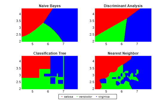
Each classification algorithm generates different decision making rules. A decision surface can help you visualize these rules.