Harmonic Analysis of Transfer Function Output

R2026b

This example finds closed-form solutions for the coefficients of frequencies in an output signal. The output signal results from passing an input through an analytical nonlinear transfer function.

This example uses the following Symbolic Math Toolbox™ capabilities:

Taylor series expansion using taylor
Formula Manipulation and Simplification

Motivation

To motivate the solution, we take a simple element from circuit theory: an ideal diode (in forward bias operation). The current, I, is the output that depends exponentially on the input, V. Diodes have found use in creating devices such as mixers and amplifiers where understanding the harmonic structure of the output can be useful in characterizing the device and meeting design specifications.

syms Is V Vo real;
I = Is*(exp(V/Vo) - 1)

I =  $Is (e^{V / Vo} - 1)$

If V is a linear combination of 2 signals at frequencies LO and RF, the nonlinear transfer function will mix LO and RF to create output with content at combinatorial harmonic frequency combinations: freqs = {LO, 2LO, RF, 2RF, LO-RF, LO-2RF,...}.

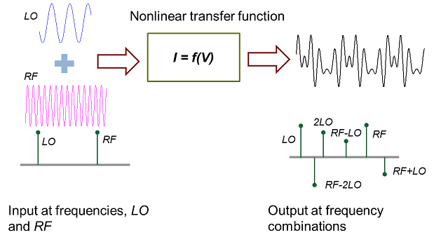
The objective of this example is to determine the coefficients of freqs in the output.

Define Input Signal

The input signal is a linear combination of two cosine signals.

syms c1 c2 t LO RF real;
input = c1*cos(LO*t) + c2*cos(RF*t)

input =  $c_{1} \cos (LO t) + c_{2} \cos (RF t)$

Define Space of Harmonic Frequency Combinations

Below, harmCombinations is a combinatorial combination of the integer multiples of the input frequencies LO and RF. We restrict the space of interest defined by 3 harmonics each in the LO and RF directions.

n = 3;
harmCombinations = [kron((0:n)',ones(n*2+1,1)),repmat((-n:n)',n+1,1)];
freqs = harmCombinations*[LO;RF];

The first n frequencies are just the negative harmonic frequencies and are therefore redundant considering that the input signal is real.

freqs = freqs(n+1:end)

freqs = 
 $(\begin{array}{c} 0 \\ RF \\ 2 RF \\ 3 RF \\ LO - 3 RF \\ LO - 2 RF \\ LO - RF \\ LO \\ LO + RF \\ LO + 2 RF \\ LO + 3 RF \\ 2 LO - 3 RF \\ 2 LO - 2 RF \\ 2 LO - RF \\ 2 LO \\ 2 LO + RF \\ 2 LO + 2 RF \\ 2 LO + 3 RF \\ 3 LO - 3 RF \\ 3 LO - 2 RF \\ 3 LO - RF \\ 3 LO \\ 3 LO + RF \\ 3 LO + 2 RF \\ 3 LO + 3 RF \end{array})$

Taylor Expansion

To cover the frequency spectrum of interest, a Taylor series of order four for I(V) is sufficient.

s = taylor(I, V, 'Order', 4)

s = 
 $\frac{Is V^{2}}{2 {Vo}^{2}} + \frac{Is V^{3}}{6 {Vo}^{3}} + \frac{Is V}{Vo}$

Use an input signal combination of the LO and RF frequencies and express f in terms of cos(LO*t) and cos(RF*t).

f0 = subs(s, V, input);
f = expand(f0)

f = 
 $\begin{array}{l} \frac{Is {c_{1}}^{2} σ_{2}}{2 {Vo}^{2}} + \frac{Is {c_{1}}^{3} {\cos (LO t)}^{3}}{6 {Vo}^{3}} + \frac{Is {c_{2}}^{2} σ_{1}}{2 {Vo}^{2}} + \frac{Is {c_{2}}^{3} {\cos (RF t)}^{3}}{6 {Vo}^{3}} + \frac{Is c_{1} \cos (LO t)}{Vo} + \frac{Is c_{2} \cos (RF t)}{Vo} + \frac{Is c_{1} c_{2} \cos (LO t) \cos (RF t)}{{Vo}^{2}} + \frac{Is c_{1} {c_{2}}^{2} \cos (LO t) σ_{1}}{2 {Vo}^{3}} + \frac{Is {c_{1}}^{2} c_{2} σ_{2} \cos (RF t)}{2 {Vo}^{3}} \\ where \\ σ_{1} = {\cos (RF t)}^{2} \\ σ_{2} = {\cos (LO t)}^{2} \end{array}$

Rewrite f in terms of single powers of cosines.

f = combine(f, 'sincos')

f = 
 $\frac{Is {c_{1}}^{2}}{4 {Vo}^{2}} + \frac{Is {c_{2}}^{2}}{4 {Vo}^{2}} + \frac{Is c_{1} \cos (LO t)}{Vo} + \frac{Is c_{2} \cos (RF t)}{Vo} + \frac{Is {c_{1}}^{2} \cos (2 LO t)}{4 {Vo}^{2}} + \frac{Is {c_{1}}^{3} \cos (LO t)}{8 {Vo}^{3}} + \frac{Is {c_{1}}^{3} \cos (3 LO t)}{24 {Vo}^{3}} + \frac{Is {c_{2}}^{2} \cos (2 RF t)}{4 {Vo}^{2}} + \frac{Is {c_{2}}^{3} \cos (RF t)}{8 {Vo}^{3}} + \frac{Is {c_{2}}^{3} \cos (3 RF t)}{24 {Vo}^{3}} + \frac{Is c_{1} {c_{2}}^{2} \cos (LO t)}{4 {Vo}^{3}} + \frac{Is {c_{1}}^{2} c_{2} \cos (RF t)}{4 {Vo}^{3}} + \frac{Is c_{1} c_{2} \cos (LO t + RF t)}{2 {Vo}^{2}} + \frac{Is c_{1} c_{2} \cos (LO t - RF t)}{2 {Vo}^{2}} + \frac{Is c_{1} {c_{2}}^{2} \cos (LO t - 2 RF t)}{8 {Vo}^{3}} + \frac{Is c_{1} {c_{2}}^{2} \cos (LO t + 2 RF t)}{8 {Vo}^{3}} + \frac{Is {c_{1}}^{2} c_{2} \cos (2 LO t + RF t)}{8 {Vo}^{3}} + \frac{Is {c_{1}}^{2} c_{2} \cos (2 LO t - RF t)}{8 {Vo}^{3}}$

Extract and Display Coefficients

Get the non-constant i.e. non-DC harmonic frequency terms of the form cos(freq*t).

cosFreqs = cos(expand(freqs*t));
terms = collect(setdiff(cosFreqs', sym(1)));

Extract the coefficients for all harmonic frequency terms including DC.

newvars = sym('x', [1,numel(terms)]);
[cx, newvarsx] = coeffs(subs(f,terms,newvars), newvars);
tx = sym(zeros(1,numel(cx)));
for k=1:numel(newvarsx)
    if newvarsx(k) ~= 1
        tx(k) = terms(newvars == newvarsx(k));
    else
        tx(k) = newvarsx(k);
    end
end
cx = simplify(cx);

Display the coefficients using table, T. Use cosFreqs as a row identifier.

cosFreqs = arrayfun(@char,cosFreqs,'UniformOutput',false);
Frequencies = arrayfun(@char,freqs,'UniformOutput',false);
Coefficients = num2cell(zeros(size(freqs)));
T = table(Frequencies,Coefficients,'RowNames',cosFreqs);

Assign cx to the appropriate rows of T corresponding to the cosine terms of tx.

nonzeroCosFreqs = arrayfun(@char,tx,'UniformOutput',false).';
T(nonzeroCosFreqs,'Coefficients') = arrayfun(@char,cx,'UniformOutput',false).';

Now, remove row names as they are redundant.

T.Properties.RowNames = {};

Observe that the expressions for the terms are symmetric in LO and RF.

T = 25×2 table
      Frequencies                      Coefficients                 
    _______________    _____________________________________________

    {'0'          }    {'(Is*(c1^2 + c2^2))/(4*Vo^2)'              }
    {'RF'         }    {'(Is*c2*(8*Vo^2 + 2*c1^2 + c2^2))/(8*Vo^3)'}
    {'2*RF'       }    {'(Is*c2^2)/(4*Vo^2)'                       }
    {'3*RF'       }    {'(Is*c2^3)/(24*Vo^3)'                      }
    {'LO - 3*RF'  }    {[                                        0]}
    {'LO - 2*RF'  }    {'(Is*c1*c2^2)/(8*Vo^3)'                    }
    {'LO - RF'    }    {'(Is*c1*c2)/(2*Vo^2)'                      }
    {'LO'         }    {'(Is*c1*(8*Vo^2 + c1^2 + 2*c2^2))/(8*Vo^3)'}
    {'LO + RF'    }    {'(Is*c1*c2)/(2*Vo^2)'                      }
    {'LO + 2*RF'  }    {'(Is*c1*c2^2)/(8*Vo^3)'                    }
    {'LO + 3*RF'  }    {[                                        0]}
    {'2*LO - 3*RF'}    {[                                        0]}
    {'2*LO - 2*RF'}    {[                                        0]}
    {'2*LO - RF'  }    {'(Is*c1^2*c2)/(8*Vo^3)'                    }
    {'2*LO'       }    {'(Is*c1^2)/(4*Vo^2)'                       }
    {'2*LO + RF'  }    {'(Is*c1^2*c2)/(8*Vo^3)'                    }
      ⋮

Verify Coefficients

As shown below, the output waveform is reconstructed from the coefficients and has an exact match with the output.

simplify(f0 - (dot(tx,cx)))

ans =  $0$

Plot Nonlinear Transfer

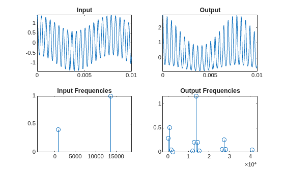
The following shows the particular nonlinear transfer function analyzed above, in the time and frequency domains, for certain values of the frequencies and voltage ratios. First, extract the data.

sample_values = struct('c1',0.4,'c2',1,'LO',800,'RF',13600,'Vo',1,'Is',1);
sample_input = subs(input,sample_values)

sample_input = 
 $\frac{2 \cos (800 t)}{5} + \cos (13600 t)$

sample_output = subs(f,sample_values)

sample_output = 
 $\frac{127 \cos (800 t)}{250} + \frac{\cos (1600 t)}{25} + \frac{\cos (2400 t)}{375} + \frac{\cos (12000 t)}{50} + \frac{\cos (12800 t)}{5} + \frac{233 \cos (13600 t)}{200} + \frac{\cos (14400 t)}{5} + \frac{\cos (15200 t)}{50} + \frac{\cos (26400 t)}{20} + \frac{\cos (27200 t)}{4} + \frac{\cos (28000 t)}{20} + \frac{\cos (40800 t)}{24} + \frac{29}{100}$

sample_freqs = zeros(size(tx));
for k=1:numel(tx)
    cosTerm = subs(tx(k),sample_values);
    freq = simplify(acos(cosTerm),'IgnoreAnalyticConstraints',true)/t;
    sample_freqs(k) = double(freq);
end
sample_heights = double(subs(cx,sample_values));

Then, use fplot and stem to plot the functions and their harmonic frequencies.

subplot(2,2,1);
fplot(sample_input,[0,0.01])
title Input
subplot(2,2,3);
stem([sample_values.LO, sample_values.RF],[sample_values.c1,sample_values.c2]);
title 'Input Frequencies'

subplot(2,2,2);
fplot(sample_output,[0,0.01])
title Output
subplot(2,2,4);
stem(sample_freqs,sample_heights)
title 'Output Frequencies'

Figure contains 4 axes objects. Axes object 1 with title Input contains an object of type functionline. Axes object 2 with title Input Frequencies contains an object of type stem. Axes object 3 with title Output contains an object of type functionline. Axes object 4 with title Output Frequencies contains an object of type stem.