Solve Algebraic Equations

Symbolic Math Toolbox™ offers both symbolic and numeric equation solvers. This topic shows you how to solve an equation symbolically using the symbolic solver solve. To compare symbolic and numeric solvers, see Select Numeric or Symbolic Solver.

Solve an Equation

If eqn is an equation, solve(eqn,x) solves eqn for the symbolic variable x.

Use the == operator to specify the familiar quadratic equation and solve it using solve.

syms a b c x
eqn = a*x^2 + b*x + c == 0;
solx = solve(eqn, x)

solx = 
$$\left(\begin{array}{c}-\frac{b+\sqrt{b^2-4\hspace{0.17em}a\hspace{0.17em}c}}{2\hspace{0.17em}a}\\ -\frac{b-\sqrt{b^2-4\hspace{0.17em}a\hspace{0.17em}c}}{2\hspace{0.17em}a}\end{array}\right)$$

solx is a symbolic vector containing the two solutions of the quadratic equation. If the input eqn is an expression and not an equation, solve solves the equation eqn == 0.

To solve for a variable other than x, specify that variable instead. For example, solve eqn for b.

solb = solve(eqn,b)

solb = 
$$-\frac{a\hspace{0.17em}{x}^2+c}{x}$$

If you do not specify a variable, solve uses symvar to select the variable to solve for. For example, solve(eqn) solves eqn for x.

Return the Full Solution to an Equation

solve does not automatically return all solutions of an equation. Solve the equation cos(x) == -sin(x). The solve function returns one of many solutions.

syms x
solx = solve(cos(x) == -sin(x),x)

solx = 
$$-\frac{\pi }{4}$$

To return all solutions along with the parameters in the solution and the conditions on the solution, set the ReturnConditions option to true. Solve the same equation for the full solution. Provide three output variables: for the solution to x, for the parameters in the solution, and for the conditions on the solution.

syms x
[solx,param,cond] = solve(cos(x) == -sin(x), x, ReturnConditions=true)

solx = 
$$\pi \hspace{0.17em}k-\frac{\pi }{4}$$

param = $$k$$

cond = $$k\in \mathbb{Z}$$

solx contains the solution for x, which is pi*k - pi/4. The param variable specifies the parameter in the solution, which is k. The cond variable specifies the condition $\mathit{k}\in \mathbb{Z}$ on the solution, which means k must be an integer. Thus, solve returns a periodic solution starting at pi/4 which repeats at intervals of pi*k, where k is an integer.

Work with the Full Solution, Parameters, and Conditions Returned by solve

You can use the solutions, parameters, and conditions returned by solve to find solutions within an interval or under additional conditions.

To find values of x in the interval -2*pi < x < 2*pi, solve solx for k within that interval under the condition cond. Assume the condition cond using assume.

assume(cond)
solk = solve(-2*pi < solx,solx < 2*pi,param)

solk = 
$$\left(\begin{array}{c}-1\\ 0\\ 1\\ 2\end{array}\right)$$

To find values of x corresponding to these values of k, use subs to substitute for k in solx.

xvalues = subs(solx,solk)

xvalues = 
$$\left(\begin{array}{c}-\frac{5\hspace{0.17em}\pi }{4}\\ -\frac{\pi }{4}\\ \frac{3\hspace{0.17em}\pi }{4}\\ \frac{7\hspace{0.17em}\pi }{4}\end{array}\right)$$

To convert these symbolic values into numeric values for use in numeric calculations, use vpa.

xvalues = vpa(xvalues)

xvalues = 
$$\left(\begin{array}{c}-3.9269908169872415480783042290994\\ -0.78539816339744830961566084581988\\ 2.3561944901923449288469825374596\\ 5.4977871437821381673096259207391\end{array}\right)$$

Visualize and Plot Solutions Returned by solve

The previous sections used solve to solve the equation cos(x) == -sin(x). The solution to this equation can be visualized using plotting functions such as fplot and scatter.

Plot both sides of equation cos(x) == -sin(x).

fplot(cos(x))
hold on
grid on
fplot(-sin(x))
title("Both sides of equation cos(x) = -sin(x)")
legend("cos(x)","-sin(x)",AutoUpdate="off")

Calculate the values of the functions at the values of x, and superimpose the solutions as points using scatter.

yvalues = cos(xvalues)

yvalues = 
$$\left(\begin{array}{c}-0.70710678118654752440084436210485\\ 0.70710678118654752440084436210485\\ -0.70710678118654752440084436210485\\ 0.70710678118654752440084436210485\end{array}\right)$$

scatter(xvalues, yvalues)

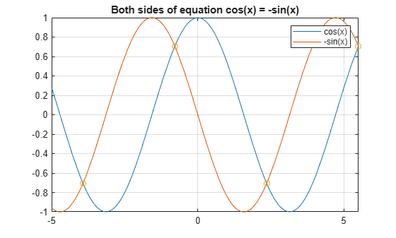
As expected, the solutions appear at the intersection of the two plots.

Simplify Complicated Results and Improve Performance

If results look complicated, solve is stuck, or if you want to improve performance, see, Choose an Approach for Solving Equations Using solve Function.