UAV Package Delivery

R2026b

This example shows how to progressively build a multicopter simulation for package delivery in a city environment. Starting with a basic waypoint mission, you integrate ground control station (GCS) connectivity, obstacle avoidance, photorealistic simulation, and a high-fidelity plant model.

Getting Started

The uavPackageDelivery.prj Simulink project file contains the reference application. The application consists of the uavPackageDelivery.slx Simulink model, its supporting files, and the project shortcuts. Open the project file by running this code.

prj = openProject('uavPackageDelivery');

Click the Getting Started project shortcut, which sets up the uavPackageDelivery.slx Simulink model for a four-waypoint mission using a low-fidelity multirotor plant model.

Model Overview

Open the uavPackageDelivery.slx Simulink model.

open_system("uavPackageDelivery");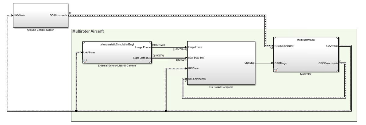

The top model consists of the following subsystems and model references:

1. Ground Control Station — Controls and monitors the aircraft while in-flight.

2. External Sensors - Lidar & Camera — Connects to a previously designed scenario or a photorealistic simulation environment. These sensors produce lidar readings from the environment as the aircraft flies through it.

3. On Board Computer — Runs algorithms intended to operate on an onboard computer independent from the autopilot.

4. Multirotor — Includes a low-fidelity and mid-fidelity multicopter model, a flight controller including its guidance logic.

The model's design data is contained in a Simulink data dictionary in the data folder (uavPackageDeliveryDataDict.sldd). Additionally, the model uses variant subsystems to manage different configurations of the model. Variables placed in the base workspace configure these variants without the need to modify the data dictionary. For more details on variant subsystems, see Variant Subsystem (Simulink).

Simulate the Waypoint Mission

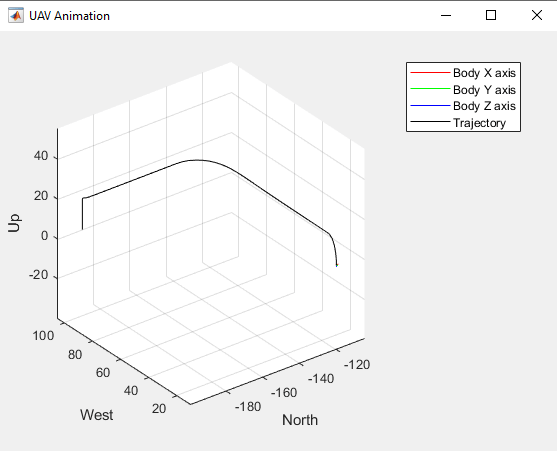
Run the uavPackageDelivery model, which shows the multirotor take off, fly, and land in a 3-D plot.

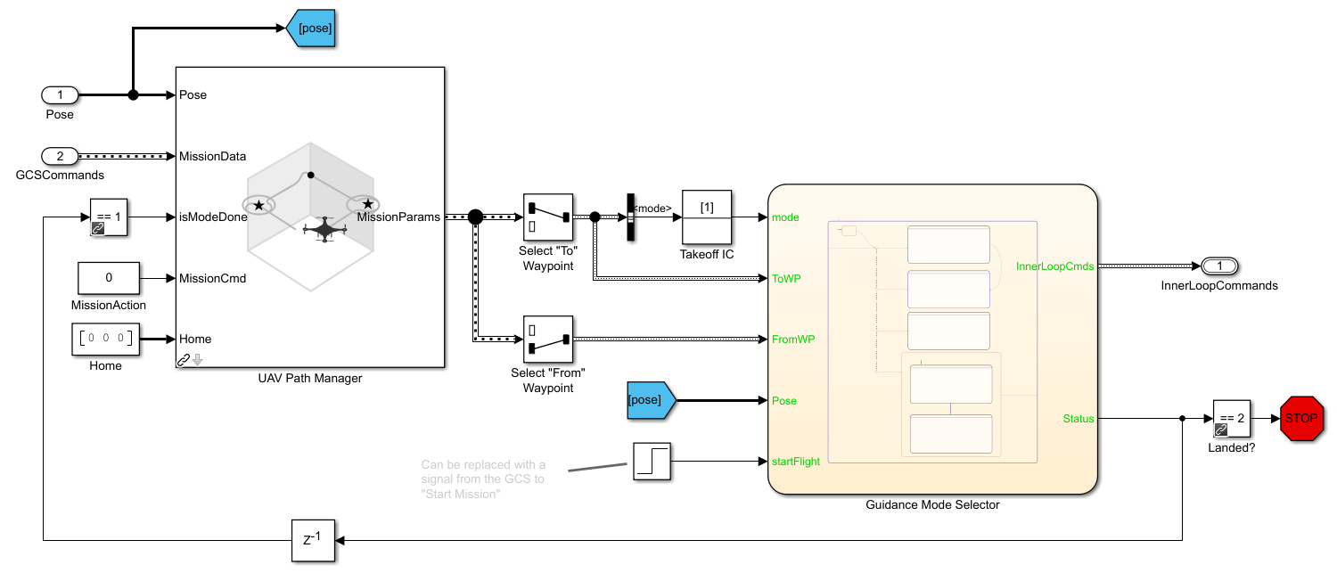
The model uses the UAV Path Manager block to determine the active waypoint throughout the flight. The active waypoint is passed into the Guidance Mode Selector Stateflow® chart to generate the necessary inner loop control commands.

Connect to a GCS

Once you can fly a basic mission, integrate your simulation with ground station software to better control the aircraft's mission. For this, you need to download and install QGroundControl Ground Control Station software.

The model uses the UAV Toolbox mavlinkio to establish a connection between Simulink and QGroundControl. The connection is implemented as a MATLAB System Block located in uavPackageDelivery/Ground Control Station/Get Flight Mission/QGC/MAVLink Interface.

To test the connectivity between Simulink and QGroundControl, follow these steps:

1. Click the Connecting to a GCS project shortcut.

2. Launch QGroundControl.

3. In QGroundControl, load the mission plan named shortMission.plan located in /utilities/qgc.

4. Run the simulation.

5. When QGroundControl indicates that it is connected to the system, upload the mission.

Once the aircraft takes off, you see the UAV fly the mission from QGroundControl, as shown below.

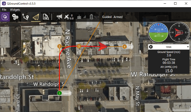
You can modify the mission by adding waypoints or moving those that are already in the mission. Upload the mission and the aircraft should respond to these changes.

Set Up the Cuboid Scenario

Now that you can fly the aircraft from a ground control station, consider the environment it flies in. This example models a few city blocks as a cuboid scenario using the uavScenario object. The scenario is based on the city block shown in the left figure below.

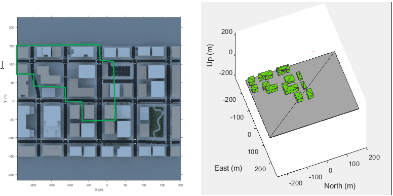
To safely fly the aircraft in this type of scenario, you need a sensor that provides information about the environment such as a lidar sensor to the model. This example uses a uavLidarPointCloudGenerator object added to the UAV scenario with a uavSensor object. The lidar sensor model generates readings based on the sensor pose and the obstacles in the environment.

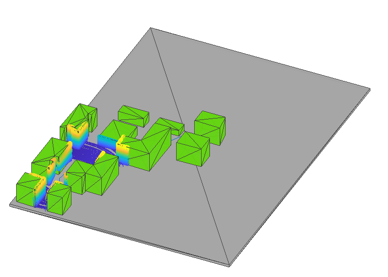
Click the Setting a Cuboid Scenario shortcut and run the model. As the model runs, a lidar point cloud image is displayed as the aircraft flies through the cuboid environment:

Configure Obstacle Avoidance

To avoid obstacles in the environment, the model must use the available sensor data as the UAV flies the mission in the environment. To modify the model configuration, click one of these shortcuts:

• Obstacle Avoidance — Configures the model to use planar lidar information and the Vector Field Histogram (Navigation Toolbox) to avoid obstacles by changing the UAV direction in the x-y plane.

• 3D Obstacle Avoidance — Configures the model to use 3D lidar points and the Obstacle Avoidance to avoid obstacles by changing the UAV direction in 3D space.

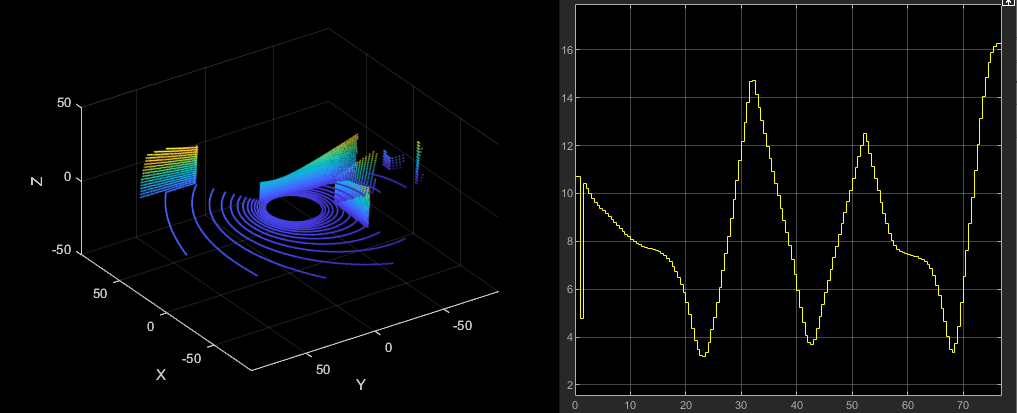
Run the model. In Obstacle Avoidance mode, as the model runs, the UAV attempts to fly in a straight path between buildings to a drop site but deviates to avoid obstacles along the way.

The image on the left shows the point cloud that is generated by the lidar sensor during the simulation. The image on the right shows the plot of closest UAV distance to buildings. When using 3D Obstacle Avoidance, the UAV adjusts its altitude during the simulation.

Simulate in Photorealistic Environment

Up to this point, the environment has been a simple cuboid scenario. To increase the fidelity of the environment, click the Photorealistic Simulation shortcut. This activates the PhotorealisticQuadrotor variant at uavPackageDelivery/photorealisticSimulationEngi/SimulationEnvironmentVariant. The variant contains blocks that configure the simulation environment and the sensors mounted on the aircraft:

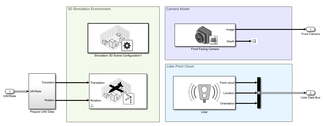
Run the model. The aircraft flies the same four-waypoint mission configured in Getting Started. As the aircraft flies the mission, the lidar point clouds update and the front-facing camera displays its image.

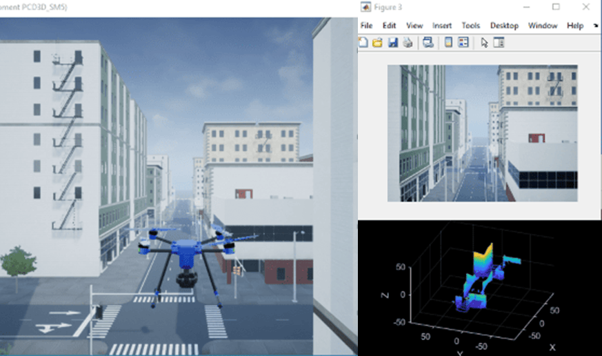
Fly Full Mission in Photorealistic Simulation Environment

Click the Fly full mission shortcut, which sets up the connectivity to QGroundControl from the Connect to a GCS section for uploading the mission inside the photorealistic environment. Follow the same steps as in Connect to a GCS to launch QGroundControl, load shortMission.plan, run the simulation, and upload the mission.

As the aircraft starts to fly, you can modify the mission in QGroundControl by adding or moving waypoints. Upload the modified mission and the aircraft responds to the changes. Throughout the flight, you see the aircraft flying in the scenario.

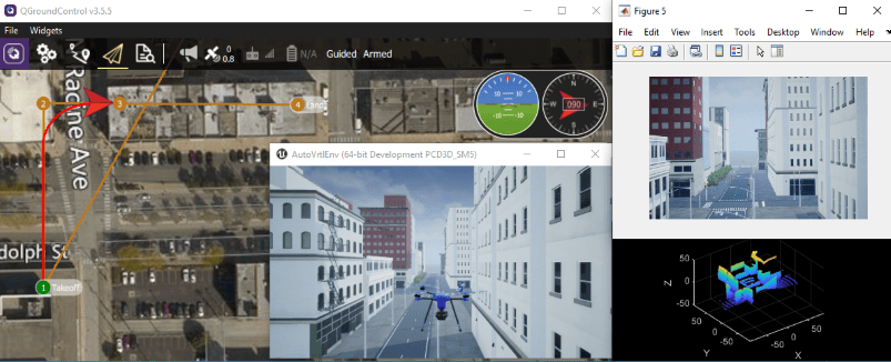
Fly with Obstacle Avoidance in Photorealistic Simulation Environment

To fly a mission with obstacle avoidance, specify a takeoff and landing point in QGroundControl and let the obstacle avoidance algorithm navigate around buildings along the path. Click the Fly full Obstacle Avoidance or Fly full 3D Obstacle Avoidance shortcut. Follow the same steps as in Connect to a GCS, but load oaMission.plan instead.

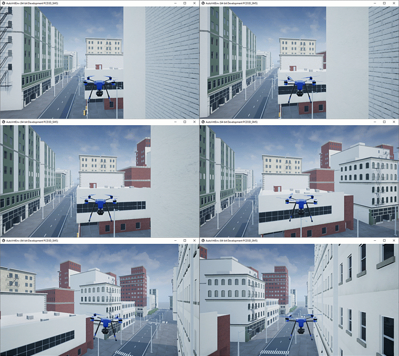
Throughout the flight, watch the aircraft try to follow the commanded path in QGroundControl, while avoiding the buildings in the environment. If you use the Fly full 3D Obstacle Avoidance shortcut, the UAV flies over the lower buildings rather than around them.

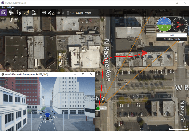
At some point during the flight, you see the UAV fly around building corners.

Add 6DOF Plant Model for Higher-Fidelity Simulation

Click the Adding a High Fidelity Plant shortcut, which activates the high-fidelity variant of the UAV model located at uavPackageDelivery/MultirotorModel/Inner Loop and Plant Model/High-FidelityModel. This variant contains an inner-loop controller and a high-fidelity plant model.

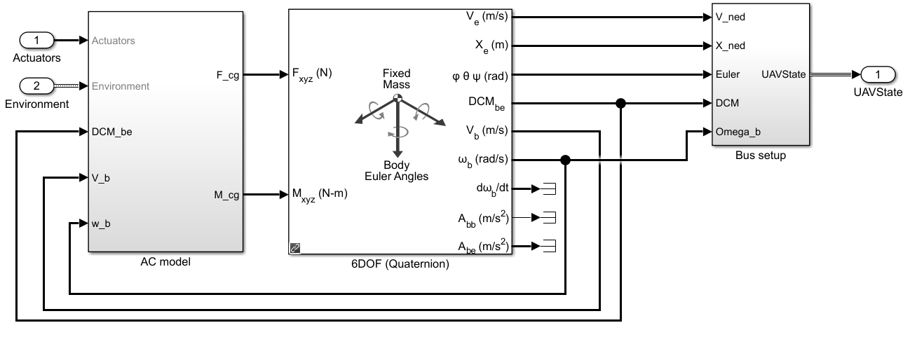
Run the model. The high-fidelity model introduces minor behavior changes, but the UAV flies the same mission.

When you are done exploring the models, close the project file.

close(prj);