Uncalibrated Stereo Image Rectification
This example shows how to use the estimateFundamentalMatrix, estimateStereoRectification, and detectSIFTFeatures functions to compute the rectification of two uncalibrated images, where the camera intrinsics are unknown.
Stereo image rectification projects images onto a common image plane in such a way that the corresponding points have the same row coordinates. This process is useful for stereo vision, because the 2-D stereo correspondence problem is reduced to a 1-D problem. As an example, stereo image rectification is often used as a preprocessing step for computing or creating anaglyph images. For more details, see the Depth Estimation from Stereo Video example.
Step 1: Read Stereo Image Pair
Read in two color images of the same scene, which were taken from different positions. Then, convert them to grayscale. Colors are not required for the matching process.
I1 = imread("yellowstone_left.png");
I2 = imread("yellowstone_right.png");

% Convert to grayscale.
I1gray = im2gray(I1);
I2gray = im2gray(I2);
Display both images side by side. Then, display a color composite demonstrating the pixel-wise differences between the images.
figure
imshowpair(I1,I2,"montage")
title("I1 (left); I2 (right)")

figure
imshow(stereoAnaglyph(I1,I2))
title("Composite Image (Red - Left Image, Cyan - Right Image)")
There is an obvious offset between the images in orientation and position. The goal of rectification is to transform the images, aligning them such that corresponding points will appear on the same rows in both images.
Step 2: Collect Interest Points from Each Image
The rectification process requires a set of point correspondences between the two images. To generate these correspondences, you will collect points of interest from both images, and then choose potential matches between them. Use detectSIFTFeatures to find blob-like features in both images.
blobs1 = detectSIFTFeatures(I1gray,ContrastThreshold=0.05);
blobs2 = detectSIFTFeatures(I2gray,ContrastThreshold=0.05);
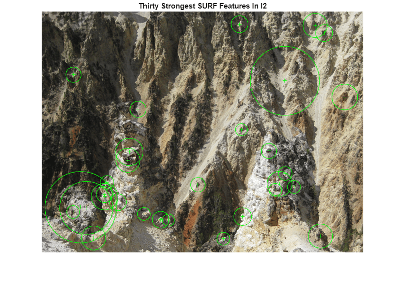
Visualize the location and scale of the thirty strongest SIFT features in I1 and I2. Notice that not all of the detected features can be matched because they were either not detected in both images or because some of them were not present in one of the images due to camera motion.
figure
imshow(I1)
hold on
plot(selectStrongest(blobs1,30))
title("Thirty Strongest SIFT Features In I1")

figure
imshow(I2)
hold on
plot(selectStrongest(blobs2,30))
title("Thirty Strongest SIFT Features In I2")

Step 3: Find Putative Point Correspondences
Use the extractFeatures and matchFeatures functions to find putative point correspondences. For each blob, compute the SIFT feature descriptors.
[features1,validBlobs1] = extractFeatures(I1gray,blobs1);
[features2,validBlobs2] = extractFeatures(I2gray,blobs2);
indexPairs = matchFeatures(features1,features2,MatchThreshold=5,Unique=true);
Retrieve locations of matched points for each image.
matchedPoints1 = validBlobs1(indexPairs(:,1),:);
matchedPoints2 = validBlobs2(indexPairs(:,2),:);
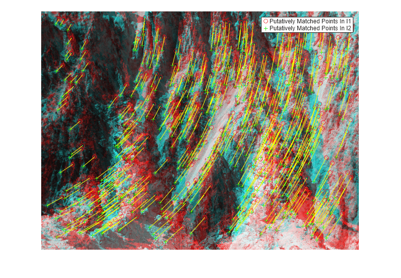
Show matching points on top of the composite image, which combines stereo images. Notice that most of the matches are correct, but there are still some outliers.
figure
showMatchedFeatures(I1, I2, matchedPoints1, matchedPoints2, 'montage')
legend("Putatively Matched Points In I1","Putatively Matched Points In I2")

Step 4: Remove Outliers Using Epipolar Constraint
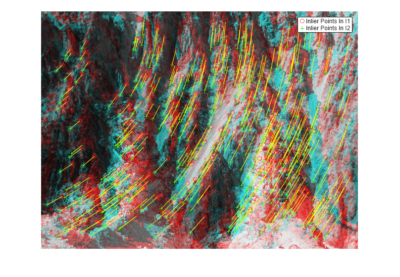
The correctly matched points must satisfy epipolar constraints. This means that a point must lie on the epipolar line determined by its corresponding point. You will use the estimateFundamentalMatrix function to compute the fundamental matrix and find the inliers that meet the epipolar constraint.
[fMatrix, epipolarInliers, status] = estimateFundamentalMatrix(...
  matchedPoints1,matchedPoints2,Method="RANSAC", ...
  NumTrials=10000,DistanceThreshold=0.1,Confidence=99.99);

if status ~= 0 || isEpipoleInImage(fMatrix,size(I1)) ...
  || isEpipoleInImage(fMatrix',size(I2))
  error(["Not enough matching points were found or "...
         "the epipoles are inside the images. Inspect "...
         "and improve the quality of detected features ",...
         "and images."]);
end

inlierPoints1 = matchedPoints1(epipolarInliers, :);
inlierPoints2 = matchedPoints2(epipolarInliers, :);

figure
showMatchedFeatures(I1, I2, inlierPoints1, inlierPoints2, 'montage')
legend("Inlier Points In I1","Inlier Points In I2")

Step 5: Rectify Images
Use the estimateStereoRectification function to compute the rectification transformations. These can be used to transform the images, such that the corresponding points will appear on the same rows.
[tform1, tform2] = estimateStereoRectification(fMatrix, ...
  inlierPoints1.Location,inlierPoints2.Location,size(I2));
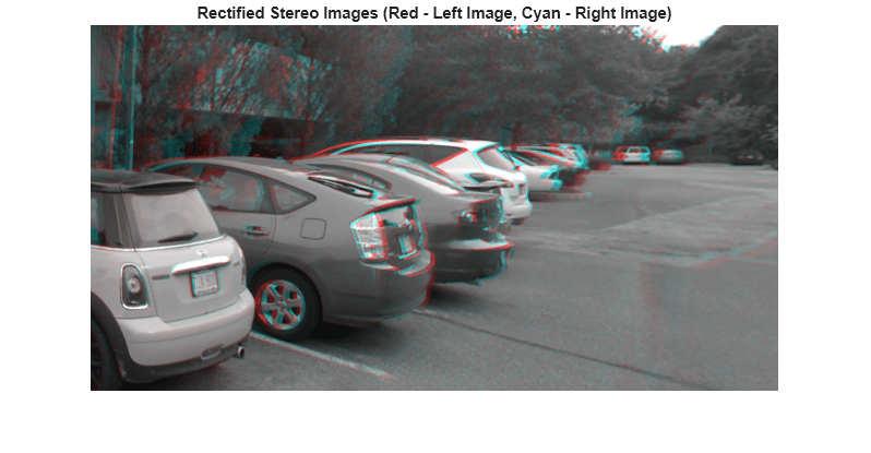
Rectify the stereo images, and display them as a stereo anaglyph. You can use red-cyan stereo glasses to see the 3D effect.
[I1Rect, I2Rect] = rectifyStereoImages(I1,I2,tform1,tform2);
figure
imshow(stereoAnaglyph(I1Rect,I2Rect))
title("Rectified Stereo Images (Red - Left Image, Cyan - Right Image)")
Step 6: Generalize The Rectification Process
The parameters used in the above steps have been set to fit the two particular stereo images. To process other images, you can use the cvexRectifyImages function, which contains additional logic to automatically adjust the rectification parameters. The image below shows the result of processing a pair of images using this function.
cvexRectifyImages("parkinglot_left.png","parkinglot_right.png");

References
[1] Trucco, E; Verri, A. "Introductory Techniques for 3-D Computer Vision." Prentice Hall, 1998.
[2] Hartley, R; Zisserman, A. "Multiple View Geometry in Computer Vision." Cambridge University Press, 2003.
[3] Hartley, R. "In Defense of the Eight-Point Algorithm." IEEE® Transactions on Pattern Analysis and Machine Intelligence, v.19 n.6, June 1997.
[4] Fischler, MA; Bolles, RC. "Random Sample Consensus: A Paradigm for Model Fitting with Applications to Image Analysis and Automated Cartography." Comm. Of the ACM 24, June 1981.