Multifractal Analysis
This example shows how to use wavelets to characterize local signal regularity. The ability to describe signal regularity is important when dealing with phenomena that have no characteristic scale. Signals with scale-free dynamics are widely observed in a number of different application areas including biomedical signal processing, geophysics, finance, and internet traffic. Whenever you apply some analysis technique to your data, you are invariably assuming something about the data. For example, if you use autocorrelation or power spectral density (PSD) estimation, you are assuming that your data is translation invariant, which means that signal statistics like mean and variance do not change over time. Signals with no characteristic scale are scale-invariant. This means that the signal statistics do not change if we stretch or shrink the time axis. Classical signal processing techniques typically fail to adequately describe these signals or reveal differences between signals with different scaling behavior. In these cases, fractal analysis can provide unique insights. Some of the following examples use pwelch for illustration. To execute that code, you must have Signal Processing Toolbox™.
Power Law Processes
An important class of signals with scale-free dynamics have autocorrelation or power spectral densities (PSD) that follow a power law. A power-law process has a PSD of the form for some positive constant, , and some exponent . In some instances, the signal of interest exhibits a power-law PSD. In other cases, the signal of interest is corrupted by noise with a power-law PSD. These noises are often referred to as colored. Being able to estimate the exponent from realizations of these processes has important implications. For one, it allows you to make inferences about the mechanism generating the data as well as providing empirical evidence to support or reject theoretical predictions. In the case of an interfering noise with a power-law PSD, it is helpful in designing effective filters.
Brown noise, or a Brownian process, is one such colored noise process with a theoretical exponent of . One way to estimate the exponent of a power law process is to fit a least-squares line to a log-log plot of the PSD.
load brownnoise
[Pxx,F] = pwelch(brownnoise,kaiser(1000,10),500,1000,1);
plot(log10(F(2:end)),log10(Pxx(2:end)))
grid on
xlabel("log10(F)")
ylabel("log10(Pxx)")
title("Log-Log Plot of PSD Estimate")
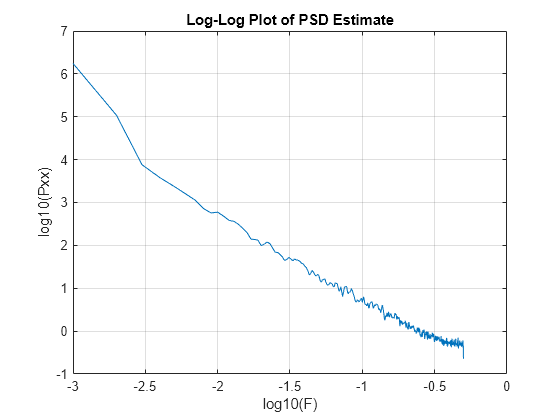
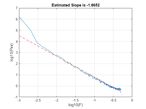
Regress the log PSD values on the log frequencies. Note you must ignore zero frequency to avoid taking the log of zero.
Xpred = [ones(length(F(2:end)),1) log10(F(2:end))];
b = lscov(Xpred,log10(Pxx(2:end)));
y = b(1)+b(2)*log10(F(2:end));
hold on
plot(log10(F(2:end)),y,"r--")
hold off
title("Estimated Slope is "+num2str(b(2)))
Alternatively, you can use both discrete and continuous wavelet analysis techniques to estimate the exponent. The relationship between the Hölder exponent, , returned by dwtleader and wtmm, and in this scenario is .
[dhbrown,hbrown,cpbrown] = dwtleader(brownnoise);
hexp = wtmm(brownnoise);
fprintf("Wavelet leader estimate is %1.2f\n",-2*cpbrown(1)-1)
Wavelet leader estimate is -1.91
fprintf("WTMM estimate is %1.2f\n",-2*hexp-1)WTMM estimate is -1.99
In this case, the estimate obtained by fitting a least-squares line to the log of the PSD estimate and those obtained using wavelet methods are in good agreement.
Multifractal Analysis
There are a number of real-world signals that exhibit nonlinear power-law behavior that depends on higher-order moments and scale. Multifractal analysis provides a way to describe these signals. Multifractal analysis consists of determining whether some type of power-law scaling exists for various statistical moments at different scales. If this scaling behavior is characterized by a single scaling exponent, or equivalently is a linear function of the moments, the process is monofractal. If the scaling behavior by scale is a nonlinear function of the moments, the process is multifractal. The brown noise from the previous section is an example of monofractal process and this is demonstrated in a later section.
To illustrate how fractal analysis can reveal signal structure not apparent with more classic signal processing techniques, load RWdata.mat which contains two time series (Ts1 and Ts2) with 8000 samples each. Plot the data.
load RWdata
plot([Ts1 Ts2])
grid on
legend("Ts1","Ts2",Location="NorthEast")
xlabel("Time")
ylabel("Amplitude")
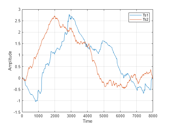
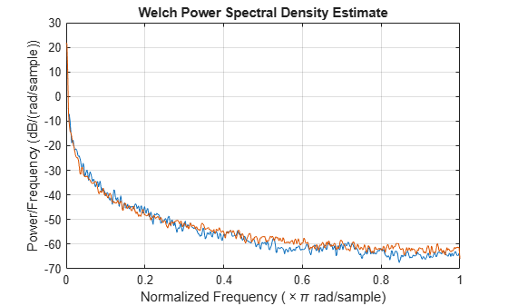
The signals have very similar second order statistics. If you look at the means, RMS values, and variances of Ts1 and Ts2, the values are almost identical. The PSD estimates are also very similar.
pwelch([Ts1 Ts2],kaiser(1e3,10))
The autocorrelation sequences decay very slowly for both time series and are not informative for differentiating the time series.
[xc1,lags] = xcorr(Ts1,300,'coef');
xc2 = xcorr(Ts2,300,'coef');
tiledlayout(2,1)
nexttile
hs1 = stem(lags(301:end),xc1(301:end));
hs1.Marker = "none";
title("Autocorrelation Sequence of Ts1")
nexttile
hs2 = stem(lags(301:end),xc2(301:end));
hs2.Marker = "none";
title("Autocorrelation Sequence of Ts2")
xlabel("Lag")
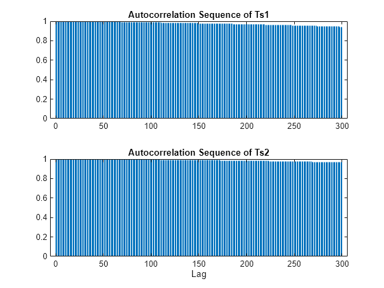
Even at a lag of 300, the autocorrelations are 0.94 and 0.96 respectively.
The fact that these signals are very different is revealed through fractal analysis. Compute and plot the multifractal spectra of the two signals. In multifractal analysis, discrete wavelet techniques based on the so-called wavelet leaders are the most robust.
[dh1,h1,cp1,tauq1] = dwtleader(Ts1);
[dh2,h2,cp2,tauq2] = dwtleader(Ts2);
figure
hp = plot(h1,dh1,"b-o",h2,dh2,"b-^");
hp(1).MarkerFaceColor = "b";
hp(2).MarkerFaceColor = "r";
grid on
xlabel("h")
ylabel("D(h)")
legend("Ts1","Ts2",Location="NorthEast")
title("Multifractal Spectrum")
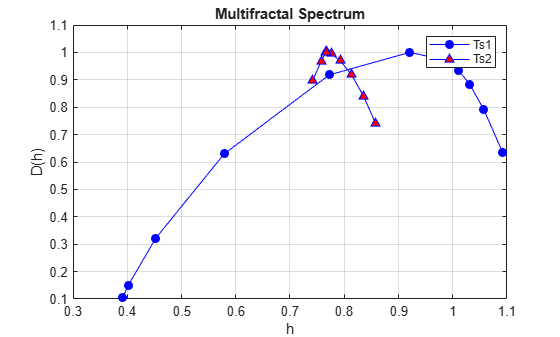
The multifractal spectrum effectively shows the distribution of scaling exponents for a signal. Equivalently, the multifractal spectrum provides a measure of how much the local regularity of a signal varies in time. A signal that is monofractal exhibits essentially the same regularity everywhere in time and therefore has a multifractal spectrum with narrow support. Conversely, A multifractal signal exhibits variations in signal regularity over time and has a multifractal spectrum with wider support. From the multifractal spectra shown here, Ts2, appears to be a monofractal signal characterized by a cluster of scaling exponents around 0.78. On the other hand, Ts1, demonstrates a wide range of scaling exponents indicating that it is multifractal. Note the total range of scaling (Hölder) exponents for Ts2 is just 0.14, while it is 4.6 times as big for Ts1. Ts2 is actually an example of a monofractal fractional Brownian motion (fBm) process with a Hölder exponent of 0.8 and Ts1 is a multifractal random walk.
You can also use the scaling exponent outputs from dwtleader along with the 2nd cumulant to help classify a process as monofractal vs. multifractal. Recall a monofractal process has a linear scaling law as a function of the statistical moments, while a multifractal process has a nonlinear scaling law. dwtleader uses the range of moments from -5 to 5 in estimating these scaling laws. A plot of the scaling exponents for the fBm and multifractal random walk (MRW) process shows the difference.
plot(-5:5,tauq1,"b-o",-5:5,tauq2,"r-^")
grid on
xlabel("Q-th Moment")
ylabel("Scaling Exponents")
title("Scaling Exponents")
legend("MRW","fBm",Location="SouthEast")
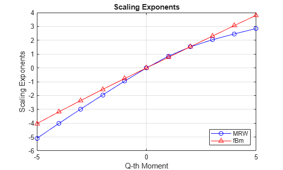
The scaling exponents for the fBm process are a linear function of the moments, while the exponents for the MRW process show a departure from linearity. The same information is summarized by the 1st, 2nd, and 3rd cumulants. The first cumulant is the estimate of the slope, in other words, it captures the linear behavior. The second cumulant captures the first departure from linearity. You can think of the second cumulant as the coefficients for a second-order (quadratic) term, while the third cumulant characterizes a more complicated departure of the scaling exponents from linearity. If you examine the 2nd and 3rd cumulants for the MRW process, they are 6 and 42 times as large as the corresponding cumulants for the fBm data. In the latter case, the 2nd and 3rd cumulants are almost zero as expected.
For comparison, add the multifractal spectrum for the brown noise computed in an earlier example.
hp = plot(h1,dh1,"b-o",h2,dh2,"b-^",hbrown,dhbrown,"r-v");
hp(1).MarkerFaceColor = "b";
hp(2).MarkerFaceColor = "r";
hp(3).MarkerFaceColor = "k";
grid on
xlabel("h")
ylabel("D(h)")
legend("Ts1","Ts2","brown noise",Location="SouthEast")
title("Multifractal Spectrum")

Where is the Process Going Next? Persistent and Antipersistent Behavior
Both the fractional Brownian process (Ts2) and the brown noise series are monofractal. However, a simple plot of the two time series shows that they appear quite different.
tiledlayout(2,1)
nexttile
plot(brownnoise)
title("Brown Noise")
grid on
axis tight
nexttile
plot(Ts2)
title("fBm H=0.8")
grid on
axis tight
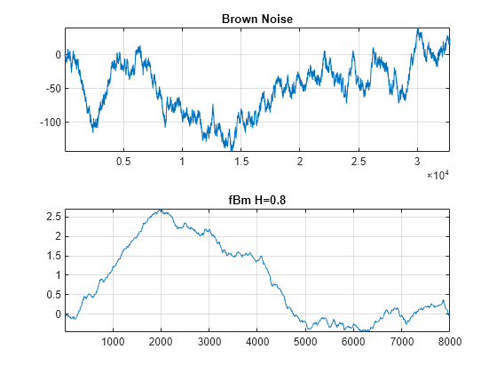
The fBm data is much smoother than the brown noise. Brown noise, also known as a random walk, has a theoretical Hölder exponent of 0.5. This value forms a boundary between processes with Hölder exponents, , from and those with Hölder exponents in the interval . The former are called antipersistent and exhibit short memory. The latter are called persistent and exhibit long memory. In antipersistent time series, an increase in value at time is followed with a decrease in value at time with a high probability. Similarly, a decrease in value at time is typically followed by an increase in value at time . In other words, the time series tends to always revert to its mean value. In persistent time series, increases in value tend to be followed by subsequent increases while decreases in value tend to be followed by subsequent decreases.
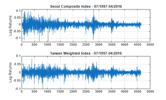
To see some real-world examples of antipersistent time series, load and analyze the daily log returns for the Taiwan Weighted and Seoul Composite stock indices. The daily returns for both indices cover the approximate period from July 1997 through April 2016.
load StockCompositeData
tiledlayout(2,1)
nexttile
plot(SeoulComposite)
title("Seoul Composite Index - 07/1997-04/2016")
ylabel("Log Returns")
grid on
nexttile
plot(TaiwanWeighted)
title("Taiwan Weighted Index - 07/1997-04/2016")
ylabel("Log Returns")
grid on
Obtain and plot the multifractal spectra of these two time series.
[dhseoul,hseoul,cpseoul] = dwtleader(SeoulComposite);
[dhtaiwan,htaiwan,cptaiwan] = dwtleader(TaiwanWeighted);
figure
plot(hseoul,dhseoul,"b-o",MarkerFaceColor="b")
hold on
plot(htaiwan,dhtaiwan,"r-^",MarkerFaceColor="r")
xlabel("h")
ylabel("D(h)")
grid on
title("Multifractal Spectrum")
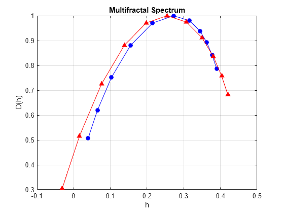
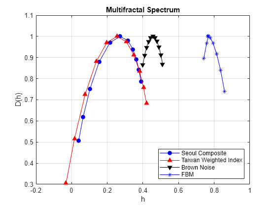
From the multifractal spectrum, it is clear that both time series are antipersistent. For comparison, plot the multifractal spectra of the two financial time series along with the brown noise and fBm data shown earlier.
plot(hbrown,dhbrown,"k-v",MarkerFaceColor="k")
plot(h2,dh2,"b-*",MarkerFaceColor="b")
legend("Seoul Composite","Taiwan Weighted Index", ...
    "Brown Noise","FBM", ...
    Location="SouthEast");
hold off
Determining that a process is antipersistent or persistent is useful in predicting the future. For example, a time series with long memory that is increasing can be expected to continue increasing. While a time series that exhibits antipersistence can be expected to move in the opposite direction.
Measuring Fractal Dynamics of Heart Rate Variability
Normal human heart rate variability measured as RR intervals displays multifractal behavior. Further, reductions in this nonlinear scaling behavior are good predictors of cardiac disease and even mortality.
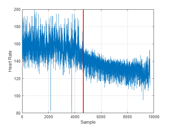
As an example of an induced change in the fractal dynamics of heart rate variability, consider a patient administered prostaglandin E1 due to a severe hypertensive episode. The data is part of RHRV, an R-based software package for heart rate variability analysis. The authors have kindly granted permission for its use in this example.
Load and plot the data. The vertical red line marks the beginning of the effect of the prostaglandin E1 on the heart rate and heart rate variability.
load hrvDrug
plot(hrvDrug)
grid on
hold on
plot([4642 4642],[min(hrvDrug) max(hrvDrug)],"r",LineWidth=2)
hold off
ylabel("Heart Rate")
xlabel("Sample")
Split the data into pre-drug and post-drug data sets. Obtain and plot the multifractal spectra of the two time series.
predrug = hrvDrug(1:4642);
postdrug = hrvDrug(4643:end);
[dhpre,hpre] = dwtleader(predrug);
[dhpost,hpost] = dwtleader(postdrug);
%figure;
hl = plot(hpre,dhpre,"b-d",hpost,dhpost,"r-^");
hl(1).MarkerFaceColor = "b";
hl(2).MarkerFaceColor = "r";
xlabel("h")
ylabel("D(h)")
grid on
legend("Predrug","Postdrug")
title("Multifractal Spectrum")
xlabel("h")
ylabel("D(h)")
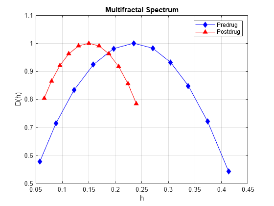
The induction of the drug has led to a 50% reduction in the width of the fractal spectrum. This indicates a significant reduction in the nonlinear dynamics of the heart as measured by heart rate variability. In this case, the reduction of the fractal dimension was part of a medical intervention. In a different context, studies on groups of healthy individuals and patients with congestive heart failure have shown that differences in the multifractal spectra can differentiate these groups. Specifically, significant reductions in the width of the multifractal spectrum is a marker of cardiac dysfunction.
References
Rodríguez-Liñares, L., A.J. Méndez, M.J. Lado, D.N. Olivieri, X.A. Vila, and I. Gómez-Conde. “An Open Source Tool for Heart Rate Variability Spectral Analysis.” Computer Methods and Programs in Biomedicine 103, no. 1 (July 2011): 39–50. https://doi.org/10.1016/j.cmpb.2010.05.012.
Wendt, Herwig, and Patrice Abry. “Multifractality Tests Using Bootstrapped Wavelet Leaders.” IEEE Transactions on Signal Processing 55, no. 10 (October 2007): 4811–20. https://doi.org/10.1109/TSP.2007.896269.
Wendt, Herwig, Patrice Abry, and Stephine Jaffard. “Bootstrap for Empirical Multifractal Analysis.” IEEE Signal Processing Magazine 24, no. 4 (July 2007): 38–48. https://doi.org/10.1109/MSP.2007.4286563.
Jaffard, Stéphane, Bruno Lashermes, and Patrice Abry. “Wavelet Leaders in Multifractal Analysis.” In Wavelet Analysis and Applications, edited by Tao Qian, Mang I Vai, and Yuesheng Xu, 201–46. Basel: Birkhäuser Basel, 2007. https://doi.org/10.1007/978-3-7643-7778-6_17.