Preprocess Data for AI-Based CSI Prediction

R2026b

Since R2026a

This example shows how to preprocess channel estimates and prepare a data set for training a gated recurrent unit (GRU) channel prediction network that enhances feedback on channel state information (CSI). It focuses on the Prepare Data step in the workflow for AI-Based CSI Feedback. You can run each step independently or work through the steps in order.

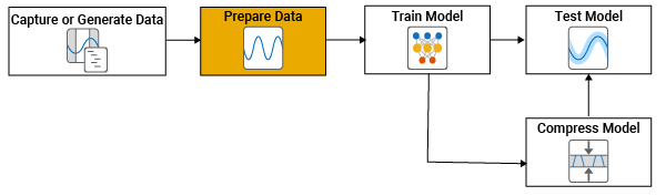
In this example, you preprocess channel realizations from previously generated data. For an example of the previous step in the workflow, see Generate MIMO OFDM Channel Realizations for AI-Based Systems.

Channel Realization Data

If the required data is not present in the workspace, this example generates the channel realization data by using the prepareChannelRealizations helper function.

maxDoppler = 5;
numSamples = 500000;
if ~exist("data","var") || ~isa(data,"signalDatastore") || ~exist("channel","var") || ~exist("carrier","var") ...
        || (exist("userParams","var") && ~strcmp(userParams.Preset,"Channel prediction"))
disp("Data not present in workspace. Running data generation code.")
    useParallel = true;
[data,systemParams,channel,carrier] = prepareChannelRealizations(numSamples,maxDoppler,useParallel);
end

Data not present in workspace. Running data generation code.

Starting parallel pool (parpool) using the 'Processes' profile ...
22-Jun-2026 11:19:49: Job Running. Waiting for parallel pool workers to connect ...
22-Jun-2026 11:20:50: Job Running. Waiting for parallel pool workers to connect ...
Connected to parallel pool with 6 workers.
Removing invalid data directory: C:\Users\user\OneDrive - MathWorks\Documents\MATLAB\ExampleManager\user.Bdoc.j3303083\5g-ex97970223\Data
Starting channel realization generation
6 worker(s) running
00:01:44 - 100% Completed

After generating the data, you can view the system configuration by inspecting outputs (data, systemParams, channel, and carrier) of the prepareChannelRealizations helper function.

Create Sequence Data

Most channel prediction neural networks require the input data to be a 3-D array structured as [features, sequence, batch], where:

Features represent channel estimates from the transmit antennas. For each antenna, the real and imaginary parts are interleaved.
Sequence corresponds to a temporal sequence of present and previous features, sampled at intervals of $Δ t$ seconds, which is usually the slot time.
Batch indexes different channel realizations.

Each feature sequence is a [ $2 N_{t x}$ , $N_{s e q u e n c e}$ ] array, where a single feature vector includes values across all transmit antennas (for a single subcarrier and receive antenna). A new sample is generated for every time step across subcarriers, receive antennas, and frames. However, the network operates on one subcarrier and one receive antenna at a time, both for input and prediction targets. The final input to the network is a [ $2 N_{t x}$ , $N_{s e q u e n c e}$ , $N_{s a m p l e s}$ ] array.

This figure shows features as columns (first dimension), sequences as rows (second dimension), and samples as pages. For speed and efficiency in MATLAB®, process samples in the highest dimension (pages dimension here).

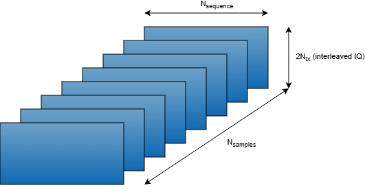
The target data is a [ $2 N_{t x}$ , 1] array, where the first dimension is the features, which are the transmit antenna channel gains at a given horizon (future time step). The final target data is a [ $2 N_{t x}$ , $N_{s a m p l e s}$ ] array.

The signalDatastore object, data, contains numFrames files, where each file holds an $H_{e s t}$ array with an [ $N_{s c}$ , $N_{s y m b o l s}$ , $N_{r x}$ , $N_{t x}$ ] channel estimate. Each frame of the channel estimates contains $N_{s y m b o l s}$ contiguous symbols per subcarrier, receiver antennas, and transmitter antennas. Read one frame and display array size.

reset(data)
Hest = read(data);
[Nsc,Nsymbol,Nrx,Ntx,Nframe] = size(Hest)

Nsc = 
624

Nsymbol = 
2492

Nrx = 
2

Ntx = 
8

Nframe = 
1

The input samples for the neural network contain $N_{s e q u e n c e}$ contiguous slots. The target samples are selected $N_{h o r i z o n}$ slots after the last training slot. As a result, $N_{s e q u e n c e}$ + $N_{h o r i z o n}$ slots are required to generate one training sample. Use a sliding window of length $N_{s e q u e n c e}$ + $N_{h o r i z o n}$ with a stride of $N_{s t r i d e}$ slots to generate training samples. Each subcarrier and receiver antenna pair in a frame results in $(N_{s y m b o l s} - (N_{s e q u e n c e} + N_{h o r i z o n} - 1)) / N_{s t r i d e}$ training samples. Choose a stride to avoid strongly correlated training samples.

maxSequenceLength = 65; % expected maximum value of Nsequence + Nhorizon in slots
symbolsPerSlot = 14;
Nstride = 10;
numSlotsPerFrame = Nsymbol/symbolsPerSlot;
samplesPerSubCarrierRx = ...
    floor((numSlotsPerFrame-maxSequenceLength+1)/Nstride);
if numSlotsPerFrame < maxSequenceLength
    error("Number of slots per frame (%d) is less than the expected maximum sequence length (%d).", ...
        numSlotsPerFrame,maxSequenceLength)
end

For channel prediction, each sample is an [ $N_{t x}$ , $N_{s e q u e n c e}$ ] array, where $N_{s e q u e n c e}$ is the number of symbols sampled at $T_{s}$ seconds, which is the slot time. Each channel estimate contains $N_{s c}$ subcarriers and $N_{r x}$ receiver antennas. Therefore, each frame results in $(N_{s y m b o l s} \div 14 - (N_{s e q u e n c e} + N_{h o r i z o n} - 1)) \times (N_{s c} N_{r x}) \div N_{s t r i d e}$ samples. Calculate the minimum number of frames required to generate numSamples training samples.

numFrames = ceil(numSamples/(samplesPerSubCarrierRx*Nsc*Nrx));
if numFrames > numel(data.Files)
    error("Not enough frames to generate %d samples. Increase number of frames to at least %d.",numSamples,numFrames)
end

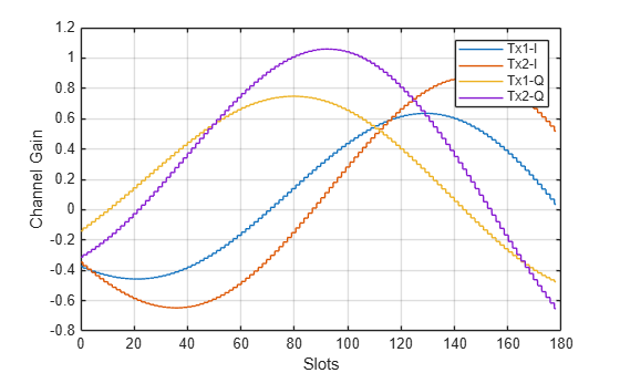
Check if the data provides enough variation in the channel for the network to learn channel characteristics. The step-wise values of the channel is a result of setting the SampleDensity property of the nrCDLChannel to a finite value.

Htemp = squeeze(Hest(1,:,1,1:2));
slots = (1:Nsymbol)/symbolsPerSlot;
plot(slots,real(Htemp))
hold("on")
plot(slots,imag(Htemp))
hold("off")
grid("on")
xlabel("Slots")
ylabel("Channel Gain")
legend("Tx1-I","Tx2-I","Tx1-Q","Tx2-Q")

Figure contains an axes object. The axes object with xlabel Slots, ylabel Channel Gain contains 4 objects of type line. These objects represent Tx1-I, Tx2-I, Tx1-Q, Tx2-Q.

Preprocess Channel Realizations

Most neural networks require the input and target data to be preprocessed and reshaped. Preprocessing reduces the neural network complexity and training time. Reshaping ensures data dimensions are interpreted correctly.

Complex-to-Real Conversion: To feed complex-valued CSI into standard neural networks, you can map each complex sample into purely real features by interleaving in-phase and quadrature components. To match the format used for the futures dimension, flatten each complex sample into the feature dimension by alternating real and imaginary values, [ℜ{x1},ℑ{x1},ℜ{x2},ℑ{x2},… ].
Add Noise: Simulate noisy channel estimates by adding white Gaussian noise.
Min-Max Normalization: Apply min-max normalization to improve training performance.
Reshape Channel Array: For autoencoder type neural networks, input and target data are the 2-D subcarrier-transmit antenna array. Temporal prediction neural networks require time series of 2-D arrays as inputs and 2-D arrays as targets.

Convert Complex Data to Real

Since the data is complex and the network requires real-valued data, separate the real and imaginary parts and store them on the last dimension.

dimSubcar = 1;
dimSymb = 2;
dimRxAnt = 3;
dimTxAnt = 4;
numDims = ndims(Hest);
dimIQ = numDims+1;
HestReal = cat(dimIQ,real(Hest),imag(Hest));

Get the dimensions of the data.

[Nsc,Nsymbol,Nrx,Ntx,Niq] = ...
size(HestReal, [dimSubcar,dimSymb,dimRxAnt,dimTxAnt,dimIQ])

Nsc = 
624

Nsymbol = 
2492

Nrx = 
2

Ntx = 
8

Niq = 
2

Reshape Data

Create a transmit antenna sample array with interleaved IQ samples as the first dimension and symbols as the second dimension. In HestReal, the symbols are time-contiguous only in the symbol dimension, which is the second dimension. Switching subcarriers, receive antennas, and frames creates discontinuities in the symbol dimension. To ensure continuity in the symbol dimension, keep the second dimension separate but combine subcarriers and receive antennas as the third dimension.

To create this array, first permute the dimensions to obtain an [ $N_{i q}$ , $N_{t x}$ , $N_{s y m}$ , $N_{s c}$ , $N_{r x}$ ] array.

H = permute(HestReal,[dimIQ dimTxAnt dimSymb dimSubcar dimRxAnt]);
disp(size(H))

           2           8        2492         624           2

Reshape the array to size [ $N_{t x} N_{i q}$ , $N_{s y m b o l}$ , $N_{o t h e r}$ ], where $N_{o t h e r}$ is $N_{s c} N_{r x}$ . Since MATLAB® reads arrays starting from the first dimension, this operation creates an array where the first dimension contains the interleaved IQ samples for the transmit antennas, the second dimension is time-contiguous symbols, and the third dimension is subcarriers and receive antennas.

Hr = reshape(H,Ntx*Niq,Nsymbol,Nsc*Nrx);
[Ntxiq,Nsymbol,Nother] = size(Hr)

Ntxiq = 
16

Nsymbol = 
2492

Nother = 
1248

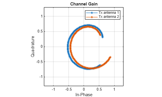
Plot the variation of the channel gain for the two transmit antennas for a random subcarrier, receive antenna, and frame.

figure()
Hsample = Hr(:,:,randi(Nsc*Nrx));
plot(Hsample(1:2:4,:)',Hsample(2:2:4,:)', '*-')
lim = floor(max(abs(Hsample),[],"all")*11)/10;
ylim([-lim lim])
xlim([-lim lim])
axis("square")
grid("on")
xlabel("In-Phase")
ylabel("Quadrature")
legend("Tx antenna 1","Tx antenna 2")
title("Channel Gain")

Figure contains an axes object. The axes object with title Channel Gain, xlabel In-Phase, ylabel Quadrature contains 2 objects of type line. These objects represent Tx antenna 1, Tx antenna 2.

Add Noise

To simulate noisy channel estimates, add noise to the channel data. Set the value for the signal-to-noise ratio (SNR).

SNR = 20;

Calculate the noise variance associated with the SNR and signal values.

$\begin{array}{l} S N R = 10 l o g_{10} (S / N) \\ \frac{S}{N} = 1 0^{(S N R / 10)} \\ N = \frac{S}{1 0^{(S N R / 10)}} \end{array}$

noiseVariance = (var(Hr,[],"all")/10^(SNR/10))/2;

Generate noisy data.

Hnoisy = Hr + randn(size(Hr),"single")*sqrt(noiseVariance);

Apply Min-Max Normalization

When you work with GRUs, input data normalization is crucial. It helps the network learn patterns more effectively, especially in time series data where values can vary significantly across different magnitudes, by ensuring all features are on a similar scale. Use min-max scaling to scale the data to a range between 0 and 1 by subtracting the minimum value and dividing by the range of the data. Check the minimum and maximum values of features.

histogram2(Hnoisy(1:2:end,:,:),Hnoisy(2:2:end,:,:),40)
grid("on")
xlabel("In-Phase Data Amplitude")
ylabel("Quadrature Data Amplitude")
zlabel("Number of Occurrences")

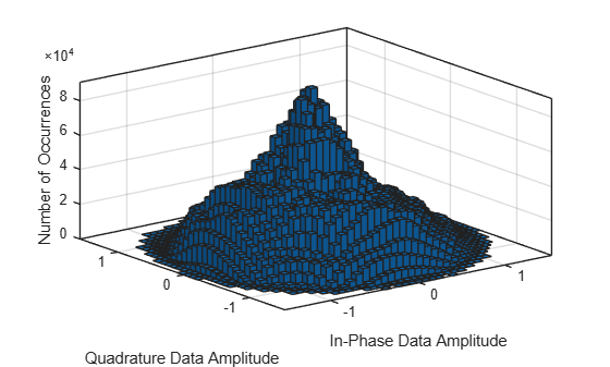
Figure contains an axes object. The axes object with xlabel In-Phase Data Amplitude, ylabel Quadrature Data Amplitude contains an object of type histogram2.

Since the histogram does not show outliers, use min-max scaling to scale the data to a range between 0 and 1 by subtracting the minimum value and dividing by the range of the data. Check the minimum and maximum values of features.

featuresMax = max(Hnoisy,[],[2 3])

featuresMax = 16×1 single column vector

    1.1091
    1.3207
    1.5275
    1.4314
    1.1073
    1.5404
    1.4428
    1.3965
    1.1859
    1.1461
    1.2489
    0.7975
    0.8585
    1.3507
    0.9847
      ⋮

featuresMin = min(Hnoisy,[],[2 3])

featuresMin = 16×1 single column vector

    -1.4619
    -1.2919
    -1.4142
    -1.4855
    -1.3917
    -1.2508
    -1.4857
    -1.5226
    -1.4961
    -1.4805
    -1.2809
    -1.4396
    -1.2450
    -1.0153
    -1.3137
      ⋮

Apply min-max scaling to the whole data set. This normalization ensures that all network inputs have a consistent scale and distribution, which can improve convergence speed and stability during training.

$f_{\max} = \max (| ℜ (H_{e s t}) |, | ℑ (H_{e s t}) |)$

$f_{\min} = \min (| ℜ (H_{e s t}) |, | ℑ (H_{e s t}) |)$

dataMax = max(featuresMax);
dataMin = min(featuresMin);

$H_{e s t} = (H_{e s t} - f_{\min}) / (f_{\max} - f_{\min}))$

Hnoisys = (Hnoisy - dataMin) / (dataMax - dataMin);
Hrs = (Hr - dataMin) / (dataMax - dataMin);

Format Input Data

The channel prediction network requires a 3-D array input, [features, sequence, batch]. The features dimension is the channel gain per transmit antenna. The sequence dimension is the symbols as a time sequence that you use in prediction, and the batch dimension is the time steps. Select the horizon value in milliseconds.

horizon = 10; % ms

Sample $N_{s e q}$ symbols from the second dimension of the Hnoisy array at $N_{t s}$ period, which contains the time-contiguous symbols. This 2-D array is the $2 N_{t x}$ -by- $N_{s e q}$ input data sample. Repeat this process for each time step in the second dimension and for each subcarrier, receiver antenna, and frame (third dimension). Since each sample requires $N_{s e q}$ previous symbols sampled at $T_{s}$ , input data can have only $N_{s y m b o l} - N_{t s} (N_{s e q} - 1)$ time-contiguous samples.

Select sequence length based on the coherence time of the channel. Compute the approximate coherence time of the channel in seconds as $T_{c} \approx \frac{0.423}{Doppler Spread}$ .

Tc = 0.423/systemParams.MaximumDopplerShift;

Calculate the coherence time in terms of slots.

numerology = (systemParams.SubcarrierSpacing/15)-1;
Tslot = 1e-3 / 2^numerology;
symbolsPerSlot = 14;
coherenceTimeInSlots = Tc / Tslot;

Set the input sequence length to 80% of the coherence time. This provides the GRU network with enough channel variation to learn temporal dynamics while keeping the sequence within one coherence period, where channel samples remain correlated. Shorter sequences also improve training efficiency and stability.

sequenceLength = ceil(coherenceTimeInSlots*0.8)

sequenceLength = 
68

Calculate the maximum data start index, number of sequences per subcarrier and receive antenna, and total number of samples you can extract from the data.

maxStart = Nsymbol-(sequenceLength+horizon)*symbolsPerSlot;
numSequencesPerChannel = floor((maxStart-1)/(Nstride*symbolsPerSlot))+1;
totalSamples = numSequencesPerChannel*Nsc*Nrx*Nframe;

First preallocate inputData as a 2 $N_{t x}$ -by- $N_{s e q}$ -by-( $N_{s y m b o l} - N_{t s} (N_{s e q} - 1)$ ) $N_{s c}$ $N_{r x}$ single precision array.

inputData = zeros(Ntxiq,sequenceLength,totalSamples,"single");

Sample the data using a for-loop over time-contiguous symbols (s), subcarriers (Nsc), receive antennas (Nrx), and frames (p). Channel samples are subject to discontinuities when the sampling process switches the number of subcarriers, receive antennas, or frames. The sequence samples must be continuous.

sample = 1;
for p = 1:Nsc*Nrx
    for s = 1:Nstride*symbolsPerSlot:maxStart
        inputData(:,:,sample) = Hnoisys(:,s:symbolsPerSlot:(s+symbolsPerSlot*(sequenceLength-1)+1),p);
        sample = sample + 1;
    end
end

Standardize the data array dimensions to align with the expected format for PyTorch® networks by permuting the data to bring time steps to the first dimension. For PyTorch coexecution examples that use the preprocessed data to train models, see Further Exploration.

inputData = permute(inputData,[3,2,1]);

Check the size of the input data array.

[Nsamples,Nsequence,Ntxiq] = size(inputData)

Nsamples = 
12480

Nsequence = 
68

Ntxiq = 
16

Check the size of the input data array in the memory.

varInfo = whos("inputData");
fprintf("inputData is %1.0f MB in memory.\n", varInfo.bytes / 2^20)

inputData is 52 MB in memory.

Format Target Data

Generate target data based on the prediction horizon. Select the setting for horizon in milliseconds. Target data contains interleaved IQ samples for transmit antennas in the first dimension and symbols on the second dimension. The targetData variable holds the channel samples that are used as target values during training.

targetData = zeros(Ntxiq,totalSamples,"single");
sample = 1;
for p = 1:Nsc*Nrx
    targetData(:,sample:sample+numSequencesPerChannel-1) = ...
        Hrs(:,1+(sequenceLength + horizon)*symbolsPerSlot:Nstride*symbolsPerSlot:end,p);
    sample = sample+numSequencesPerChannel;
end

Permute targetData to bring time steps to the first dimension.

targetData = permute(targetData,[2,1]);
size(targetData)

ans = 1×2

    12480    16

You can now preprocess the data in bulk or preprocess it using a transform datastore.

Preprocess Data in Bulk

The helperPreprocess3GPPChannelData helper function preprocesses the channel realizations saved in files in the dataDir directory. The helper function takes the sdsChan signal datastore as its first input to load the channel realizations and optionally saves the preprocessed data to the processed folder in the dataDir directory.

Set TrainingObjective to "prediction" to generate preprocessed channel realizations that you can use as the input signal and the target signal of a prediction neural network. Set AverageOverSlots to false. To disable truncation in the delay domain, set TruncateChannel to false. If you have Parallel Computing Toolbox, you can read and preprocess the data in parallel.

useParallel = true;
sdsPreprocessed = helperPreprocess3GPPChannelData( ...
data, ...
TrainingObjective="prediction", ...
AverageOverSlots=false, ...
TruncateChannel=false, ...
InputSequenceLength=sequenceLength, ...
PredictionWindowStride=Nstride, ...
PredictionHorizon=horizon, ...
AddNoise=true, ...
SNR=SNR, ...
DataComplexity="real (interleaved)", ...
DataDomain="Frequency-Spatial (FS)", ...
UseParallel=useParallel, ...
SaveData=true);

Starting CSI data preprocessing
6 worker(s) running
00:00:37 - 100% Completed

processedData = readall(sdsPreprocessed);
inputCells = cellfun(@(C) C{1},processedData,UniformOutput=false);
targetCells = cellfun(@(C) C{2},processedData,UniformOutput=false);
inputData = cat(3, inputCells{:});
targetData = cat(2, targetCells{:});
whos("inputData","targetData")

  Name             Size                        Bytes  Class     Attributes

  inputData       16x68x461760            2009579520  single              
  targetData      16x461760                 29552640  single

Apply min-max normalization.

dataMax = max(inputData,[],"all")

dataMax = single

3.3223

dataMin = min(inputData,[],"all")

dataMin = single

-2.9007

inputData = (inputData - dataMin) / (dataMax - dataMin);
targetData = (targetData - dataMin) / (dataMax - dataMin);

Save the normalization parameters.

dataOptions.Normalization = "min-max";
dataOptions.MinValue = dataMin;
dataOptions.MaxValue = dataMax;

Preprocess Data Using Transform Datastore

Alternatively, preprocess the data using a transform datastore, where the transform function is the preconfigured helperPreprocess3GPPChannelData function. Normalize the data using the previously determined the minimum and maximum normalization parameters. The transform function creates a new datastore, tdsChan, that applies preprocessing to the data read from the underlying datastore, sdsChan. This preprocessing method is particularly useful when dealing with large data sets that cannot fit entirely in memory. If you have Parallel Computing Toolbox, you can read and preprocess the data in parallel. Set UseParallel must be set to true in the readall function. Since Parallel Computing Toolbox does not support nested parallel loops, UseParallel must be set to false when calling helperPreprocess3GPPChannelData in a transform datastore.

tdsChan = transform(data, @(x){helperPreprocess3GPPChannelData( ...
    x, ...
    TrainingObjective="prediction", ...
    AverageOverSlots=false, ...
    TruncateChannel=false, ...
    InputSequenceLength=sequenceLength, ...
    PredictionWindowStride=Nstride, ...
    PredictionHorizon=horizon, ...
    AddNoise=true, ...
    SNR=SNR, ...
    DataComplexity="real (interleaved)", ...
    DataDomain="Frequency-Spatial (FS)", ...
    SaveData=false, ...
    UseParallel=false, ...
    Verbose=false, ...
    Normalization="min-max", ...
    MinimumValue=dataOptions.MinValue, ...
    MaximumValue=dataOptions.MaxValue)});

Read all the data and apply preprocessing.

dataCell = readall(tdsChan,UseParallel=useParallel);
inputCells = cellfun(@(C) C{1},dataCell,UniformOutput=false);
targetCells = cellfun(@(C) C{2},dataCell,UniformOutput=false);
inputData2 = cat(3, inputCells{:});
targetData2 = cat(2, targetCells{:});
whos("inputData2","targetData2")

  Name              Size                        Bytes  Class     Attributes

  inputData2       16x68x461760            2009579520  single              
  targetData2      16x461760                 29552640  single

Further Exploration

After preprocessing channel realizations, you can use the CSI snapshots to explore channel prediction neural network training in these examples:

Train PyTorch Channel Prediction Models — Design, train, and evaluate temporal models that predict future channel realizations from past snapshots.
Train PyTorch Channel Prediction Models with Online Training — Design, train, and evaluate temporal models that predict future channel realizations from past snapshots in an online fashion.

For information about the full workflow, see AI-Based CSI Feedback.

Local Functions

function [sdsChan,systemParams,channel,carrier] = prepareChannelRealizations(numSamples,maxDoppler,useParallel)
% prepareChannelRealizations Generate channel realizations for prediction

maxHorizon = 100;
carrier = nrCarrierConfig;
nSizeGrid = 52; % Number resource blocks (RB)
systemParams.SubcarrierSpacing = 15;
carrier.NSizeGrid = nSizeGrid;
carrier.SubcarrierSpacing = systemParams.SubcarrierSpacing;
Nsc = 12*nSizeGrid;
systemParams.DelaySpread = 300e-9; % s
systemParams.DelayProfile = "CDL-C";
systemParams.TxAntennaSize = [2 2 2 1 1]; % [M N P Mg Ng] rows, columns, polarizations, row panels, column panels
systemParams.RxAntennaSize = [2 1 1 1 1];
systemParams.MaximumDopplerShift = maxDoppler; % Hz
systemParams.Carrier = carrier;
channel = helper3GPPChannel(systemParams);

chanInfo = info(channel);
Nrx = chanInfo.NumReceiveAntennas;

Tc = 0.423/systemParams.MaximumDopplerShift;
numerology = (systemParams.SubcarrierSpacing/15)-1;
Tslot = 1e-3 / 2^numerology;
coherenceTimeInSlots = Tc / Tslot;
sequenceLength = ceil(coherenceTimeInSlots*0.8);
numSlotsPerFrame = sequenceLength + maxHorizon + 10;
stride = 10;
samplesPerSubCarrierRx = floor((numSlotsPerFrame-sequenceLength+1)/stride);
numFrames = ceil(numSamples / (samplesPerSubCarrierRx*Nrx*Nsc));

saveData = true;
dataDir = fullfile(pwd,"Data");
dataFilePrefix = "nr_channel_est";
resetChannel = true;
sdsChan = helper3GPPChannelRealizations(...
    numFrames, ...
    channel, ...
    carrier, ...
    UseParallel=useParallel, ...
    SaveData=saveData, ...
    DataDir=dataDir, ...
    DataFilePrefix=dataFilePrefix, ...
    NumSlotsPerFrame=numSlotsPerFrame, ...
    ResetChannelPerFrame=resetChannel);
end