Mobility Modeling with Ray Tracing Channel
This example shows how to use a ray tracing channel to model mobility in a communications link.
Introduction
Most modern communications systems allow motion of one or both ends of the link. Often the cellular user equipment (UE) is in motion as it communicates with a base station (BS). The UE may require a handoff from one BS to the next as motion continues across cell sectors or cells. Similar phenomena occur when someone carries a laptop through a building. The laptop stays connected to fixed WiFi® network infrastructure in the building by handing off to different access points.
This example shows you how to define a path in an environment of interest. The environment can be a geo-based map, a building plan, or a drawing of a room. Within any of these environments, you can define critical waypoints and the path between those waypoints. At waypoints, the entity may stop, start, turn, pause, change speed, or have some other adjustment of its path. Given the overall path, ray tracing computes a sequence of channel models corresponding to the chosen path. You can incorporate these channel models into a second pass to do a link-level or system-level simulation.
In this example, you define the granularity of channel model computation along the path as an input parameter to the computeWaypoints local function. After defining the route, you use the raytrace function to do ray tracing analysis at each waypoint and then construct the corresponding channel using a comm.RayTracingChannel System object™ for use in a link-level simulation. This example does not address issues of spatial consistency or any kind of channel model continuity along the path. At each point along the path, you recompute the channel model by analyzing the scene from that point in time without regard to any results from the previous analysis point. At the end of this example, you incorporate the computed channel models into a simplified OFDM-MIMO transmission and run in a link-level simulation.
Set Up Route
Import Map Data
This example uses an OpenStreetMap® file (northeastern.osm) that corresponds to a portion of downtown Boston. The file is downloaded from https://www.openstreetmap.org, which provides access to crowd-sourced map data all over the world. The data is licensed under the Open Data Commons Open Database License (ODbL), https://opendatacommons.org/licenses/odbl/. Import the buildings information from the OpenStreetMap file and visualize it in Site Viewer.
sv = siteviewer( ...
    Buildings="northeastern.osm", ...
    Basemap="satellite");
Create UE Antenna Array
Configure a 5G antenna phased array for a carrier frequency of 5.8 GHz, which is typical for cellular systems.
fc = 5.8e9;
c = physconst("LightSpeed");
lambda = c/fc;

ueElement = phased.NRAntennaElement(PolarizationAngle = 45);
ueArray = phased.NRRectangularPanelArray( ...
    Size=[1 1 1 1], ...
    ElementSet={ueElement}, ...
    Spacing=lambda*[.5 .5 1 1]);
Create UE Receiver Sites Along Route
Specify a route by setting a few waypoints on a major road and creating a straight line path between the waypoints. You can obtain the initial control points by manually right-clicking the map in Site Viewer to get latitude and longitude coordinates for start point, stop point, and any turn points. These coordinates define the mobile paths in the simulation.
For this example, the specified route is in Boston along Huntington Avenue from Gainsborough Street toward Forsyth Street in front of Northeastern University and stopping just before the Boston Museum of Fine Arts.
route.controlPoints.lats = [42.341482 42.341102 42.339903];
route.controlPoints.lons = [-71.086650 -71.087238 -71.090416];
route.controlPoints.heights = [1.5 1.5 1.5];
route.spacing = 5;

controlpts = txsite( ...
    Latitude=route.controlPoints.lats, ...
    Longitude=route.controlPoints.lons, ...
    AntennaHeight=route.controlPoints.heights);
Use the computeWaypoints local function to define the route by starting at one end and then moving on a straight line between the waypoints specified above, estimating the channel all along the route with granularity defined by route.spacing. This function does not check the viability of the path in the real world, so manually verify that no points are in illogical locations, such as inside a building or on a lamp post. Assuming that the straight line path is valid, you can use this local function to determine the intermediate waypoints from the initial manually defined stop, start, and turn waypoints.
rxs = computeWaypoints(controlpts,route.spacing,ueArray);
Compute total distance along route.
totdist = 0;
for i=1:numel(controlpts)-1
    totdist = totdist + distance(controlpts(i),controlpts(i+1));
end
disp("Total distance along route is " + totdist + " meters.");
Total distance along route is 358.0733 meters.
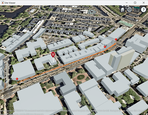
Visualize Route
Show the control points and UE receiver sites.
show(controlpts, ...
    ShowAntennaHeight=false, ...
    Icon="pin.png", ...
    IconSize=[12 30])
show(rxs, ...
    ShowAntennaHeight=false, ...
    Icon="OrangeDot.png", ...
    IconSize=[5 5])
Capture the current perspective by using camera functions. You use these functions later to hold this perspective.
[camlat,camlon,camheight] = campos(sv);
cpitch = campitch(sv);
cheading = camheading(sv);
Create Base Station Antenna Array
Configure the BS antenna array as a single four-element rectangular panel array.
gNBElement = phased.NRAntennaElement( ...
    PolarizationAngle=-45, ...
    Beamwidth=120);
bsArray = phased.NRRectangularPanelArray( ...
    Size=[2 2 1 1], ...
    ElementSet={gNBElement}, ...
    Spacing=lambda*[.5 .5 1 1]);
Create Base Station Transmitter Site
Add the base station to the top of a building that sits adjacent to the specified route.
tx = txsite(Name="NR5G", ...
    Latitude=42.3405645965253, ...
    Longitude=-71.0892925339939, ...
    Antenna=bsArray, ...
    AntennaHeight=17, ...
    TransmitterFrequency=fc);
show(tx);

campos(sv,camlat,camlon,camheight);
campitch(sv,cpitch);
camheading(sv, cheading);
Perform Ray Tracing Analysis and Visualization
Compute Rays and Received Signal Strength Along Route
When computing signal strength along the route, you must use the ray tracing or Longley-Rice propagation models to account for the attributes of the scene. In this example, you use the sigstrength function to compare the signal strength along the route for ray tracing and Longley-Rice propagation models. Even though the Longley-Rice propagation model is not well suited to this scenario (because the receiver and transmitter are too close to each other), it provides a point of reference. For most of the route (after the first 50 meters), the agreement between the predicted received signal strength for Longley-Rice and for ray tracing propagation models is reasonable. Because the code in this section conducts a complete ray tracing analysis at each waypoint, it can take a while to execute. You can reduce the time by increasing the spacing between waypoints (route.spacing).
Create the propagation models. The ray tracing propagation model includes propagation paths with up to 2 reflections and 1 diffraction. In addition, it drops any path with more than 20 dB loss below the strongest path.
numreflecs = 2;
numdiffracs = 1;
maxrelpathloss = 20;
% Use GPU for raytracing if available
rtpropmdl = propagationModel("raytracing", ...
    MaxNumReflections=numreflecs, ...
    MaxNumDiffractions=numdiffracs, ...
    MaxRelativePathLoss=maxrelpathloss, ...
    UseGPU="auto");

longricepropmdl = propagationModel("longley-rice");
Typically, beamforming and tracking are important features of this kind of simulation because they keep the transmit and receive antenna arrays pointed at each other while the BS and UE motion occurs. For the sake of simplicity, this example repoints the antenna main beam of the BS and UE towards each other at each computation point. Use the computeSigStrengthFromRays local function to compute signal strengths from rays.
numrxs = numel(rxs);
for i = 1:numrxs
    tx.AntennaAngle = angle(tx,rxs(i));
    rxs(i).AntennaAngle = angle(rxs(i), tx);
    rrays{i} = raytrace(tx,rxs(i),rtpropmdl); %#ok<*SAGROW>
    rlos(i) = los(tx,rxs(i));

    rssrt(i) = computeSigStrengthFromRays(rrays{i},tx,rxs(i),fc);
    rsslongrice(i) = sigstrength(rxs(i),tx,longricepropmdl);
end
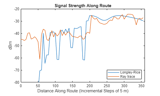
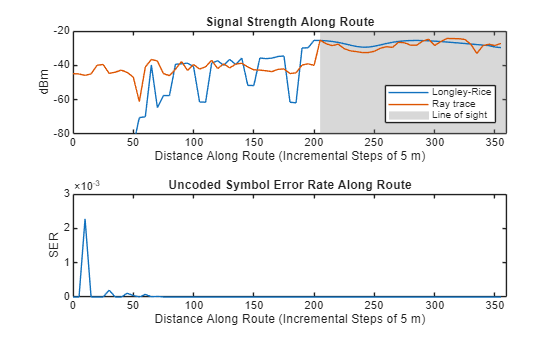
Plot Received Signal Strength Along Route
xpts = 0:(route.spacing):totdist;
figure
tiledlayout("vertical")
nexttile
plot(xpts,rsslongrice,xpts,rssrt);
xlim([0 360]); ylim([-80 -20])
title("Signal Strength Along Route")
xlocations = sprintf("Distance Along Route (Incremental Steps of %g m)",route.spacing);
xlabel(xlocations)
ylabel("dBm")
legend("Longley-Rice","Ray trace", Location="southeast")
Analyze Impact of Line-of-Sight
Focusing on the ray tracing signal strength results, you can see two distinct regions on the plot, the first section averaging around 40 dB and the second section averaging around 30 dB. To gain insight into the 10 dB difference, perform ray tracing for a point or two on either side of the transition.
d1 = 285; % meters
rx1idx = floor((d1/totdist)*numrxs);
plot(rrays{rx1idx}{1})
rssrt1 = rssrt(rx1idx)
rssrt1 = -28.2437
d2 = 20; % meters
rx2idx = floor((d2/totdist)*numrxs);
plot(rrays{rx2idx}{1})
rssrt2 = rssrt(rx2idx)
rssrt2 = -44.9810
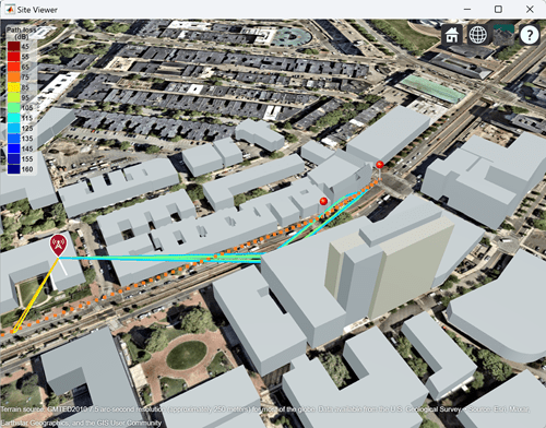
From the plots of the rays for these two locations, you can see that the first case requires a bounce or two whereas the second case has a clear path between transmitter and receiver. As shown by the signal strength plot, the color of the second set of rays indicates a stronger received signal than the first set of rays.
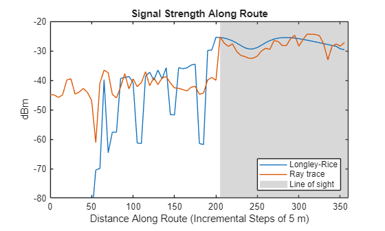
You can also analyze line-of-sight access between the transmitter and the moving receiver to see the same result. For this scenario, the middle of the route has one transition. Before that transition there is no line-of-sight access, but after the transition there is line-of-sight.
firstlos = 1;
while rlos(firstlos) == 0
    firstlos = firstlos + 1;
end
xr = xregion(xpts(firstlos),Inf);
xr.DisplayName = "Line of sight";
Simulate Communications Link
Compute Channel Models
Now compute a set of channel models appropriate for use in link-level or system-level simulation so that you can analyze the performance of the link or links along the route. You construct these channel models using the earlier ray tracing results.
Configure the channel models to have a sample rate of 30.72 MHz, which is typical for 5G systems. This sample rate must match the rate for link-level configuration.
fs = 30.72e6;
channels = cell(1,numrxs);
for i = 1:numrxs
    tx.AntennaAngle = angle(tx,rxs(i));
    chan = comm.RayTracingChannel(rrays{i}{1},tx,rxs(i));
    chan.SampleRate = fs;
    chan.NormalizeImpulseResponses = false;
    chan.NormalizeChannelOutputs = false;
    channels{i} = chan;
end
Model Communications Link Along Prescribed Route
Having derived a sequence of channel models, you are now equipped to use that sequence of channel models in a link-level or system-level simulation to characterize performance as the UE moves along the prescribed route.
For example, if you specify a UE speed of 50 km/hr to model someone talking on the cell phone as they drive along a city street and you update the channel model every 5 m along the path, then you must change to the next channel model in the sequence every 5 m / (50 * 1000 m / 3600 s), which yields 360 ms per 5 m along the path. As simulation time advances, you must update the channel to the next time step in the sequence every 360 milliseconds. This example ignores potential channel continuity impact (such as spatial consistency) required for accuracy as the channel model morphs along the path. This part of the simulation can also take a while to execute. Along with the ray trace spacing, the UE speed as it moves along the route determines how much data runs through the link and the simulation duration. The default speed of 100 km/hr is high for a city street, but it is a starting point to shorten the overall simulation time. The hMIMOLinkfcn helper function processes the OFDM MIMO link and outputs the hard decision probability of error for each point along the route.
ueSpeedKmPerHr = 100;
ueSpeed = ueSpeedKmPerHr * 1000 / 3600; % Meters per second
timePerWpt = route.spacing / ueSpeed;
perr = zeros(1,numel(channels));
for i = 1:numel(perr)
    perr(i) = hMIMOLinkfcn(timePerWpt,channels{i}, bsArray.getNumElements);
end

nexttile
plot(xpts,perr)
xlim([0 360]); ylim([0 .003])
title("Uncoded Symbol Error Rate Along Route")
xlabel(xlocations)
ylabel("SER")
Local Functions
The computeWaypoints local function computes waypoints between control points on a map and returns rxsite objects at those waypoints.
function wayptRxsites = computeWaypoints(controlPts,spacing,ueArray)
theDist = 0;
myDist = 0;
idx = 0;
offset = 0;
rxs = rxsite.empty;
for sgmntIdx = 1 : numel(controlPts)-1 % Road segment
    theDist = theDist + ...
        distance(controlPts(sgmntIdx),controlPts(sgmntIdx+1));
    az = angle(controlPts(sgmntIdx),controlPts(sgmntIdx+1));
    [lat,lon] = location(controlPts(sgmntIdx),offset,az);
    % Set next point on this segment
    idx = idx + 1;
    locname = sprintf(" P%d",idx);
    rxs(idx) = rxsite(Name=locname, ...
        Latitude=lat, Longitude=lon, Antenna=ueArray, ...
        AntennaHeight=controlPts(sgmntIdx).AntennaHeight);
    myDist = myDist + spacing;
    while myDist+offset < theDist
        % Next point on current segment
        [lat,lon] = location(rxs(idx),spacing,az);
        idx = idx+1;
        % Set next point on this segment
        locname = sprintf("P%d",idx);
        rxs(idx) = rxsite(Name=locname, ...
            Latitude=lat, Longitude=lon, Antenna=ueArray, ...
            AntennaHeight=controlPts(sgmntIdx).AntennaHeight);
        myDist = myDist + spacing;
    end
    offset = myDist - theDist;
end
wayptRxsites = rxs;
end
The computeSigStrengthFromRays local function computes signal strengths from rays. This function avoids recalculation of rays which improves run-time performance.
function ss = computeSigStrengthFromRays(rays,tx,rx,fc)
N11 = length(rays{1});
linRxPWRtmp = 0;
dbP1Tpwr = 10 * log10(tx.TransmitterPower);
azTxToRx = [];
elTxToRx = [];
azRxToTx = [];
elRxToTx = [];
for i = 1:N11
    azTxToRx(i) = ...
        rem(rays{1}(i).AngleOfDeparture(1) - tx.AntennaAngle,180);
    elTxToRx(i) = rays{1}(i).AngleOfDeparture(2);
    azRxToTx(i) = ...
        rem(rays{1}(i).AngleOfArrival(1) - rx.AntennaAngle,180);
    elRxToTx(i) = rays{1}(i).AngleOfArrival(2);
end
txPatternGain = directivity(tx.Antenna,fc,[azTxToRx; elTxToRx]);
rxPatternGain = directivity(rx.Antenna,fc,[azRxToTx; elRxToTx]);
for i = 1:N11
    % +30 to convert to dBm
    dbRxPWR_i = dbP1Tpwr + 30 + txPatternGain(i) + ...
        rxPatternGain(i) - rays{1}(i).PathLoss;
    linRxPWRtmp = linRxPWRtmp + ...
        exp(1i*rays{1}(i).PhaseShift) * 10^(dbRxPWR_i/20);
end
estTotPwr11 = 20 * log10(abs(linRxPWRtmp));
ss = estTotPwr11;
end
See Also
Objects
comm.RayTracingChannel|phased.NRRectangularPanelArray(Phased Array System Toolbox) |propagationModel|raytrace