Tune Phase-Locked Loop Using Loop-Shaping Design
This example shows how to tune the components of a passive loop filter to improve the loop bandwidth of a phase-locked loop (PLL) system. To obtain a desired loop frequency response, this example computes the loop filter parameters using the fixed-structure tuning methods provided in the Control System Toolbox™ software. The PLL system is modeled using a reference architecture block from the Mixed-Signal Blockset™ library.
Introduction
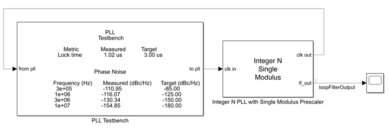
A PLL is a closed-loop system that produces an output signal whose phase depends on the phase of its input signal. The following diagram shows a simple model with a PLL reference architecture block (Integer N PLL with Single Modulus Prescaler (Mixed-Signal Blockset)) and a PLL Testbench (Mixed-Signal Blockset) block.
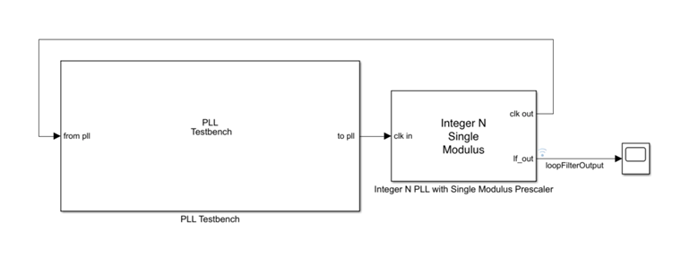
The closed-loop architecture inside the PLL block consists of a phase-frequency detector (PFD), charge pump, loop filter, voltage controlled oscillator (VCO), and prescaler.
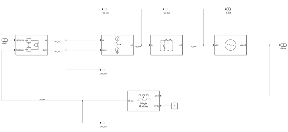
The Mixed-Signal Blockset library provides multiple reference architecture blocks to design and simulate PLL systems in Simulink®. You can tune the components of the Loop Filter (Mixed-Signal Blockset) block, which is a passive filter, to get the desired open-loop bandwidth and phase margin.
Using the Control System Toolbox software, you can specify the shape of the desired loop response and tune the parameters of a fixed-structure controller to approximate that loop shape. For more information on specifying a desired loop shape, see Loop Shape and Stability Margin Specifications. In the preceding PLL architecture model, the loop filter is defined as a fixed-order, fixed-structure controller. To achieve the target loop shape, the values of the resistances and capacitances of the loop filter are tuned. Doing so improves the open-loop bandwidth of the system and, as a result, reduces the measured lock time.
Set Up Phase-Locked Loop Model
Open the model.
model = 'PLL_TuneLoopFilter';
open_system(model)
The PLL block uses the configuration specified in Design and Evaluate Simple PLL Model (Mixed-Signal Blockset) for the PFD, Charge pump, VCO, and Prescalar tabs in the block parameters. The Loop Filter tab specifies the type as a fourth-order filter, and sets the loop bandwidth to 100 kHz and phase margin to 60 degrees. The values for the resistances and capacitances are automatically computed.
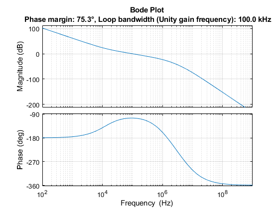
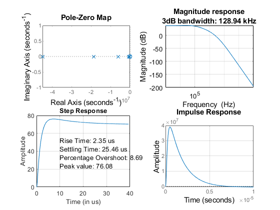
To observe the current loop dynamics of the PLL, in the block parameters, on the Analysis tab, select Open Loop Analysis and Closed Loop Analysis. The unity gain frequency is 100 kHz. The closed-loop system is stable and the 3-dB bandwidth is 128.94 kHz.
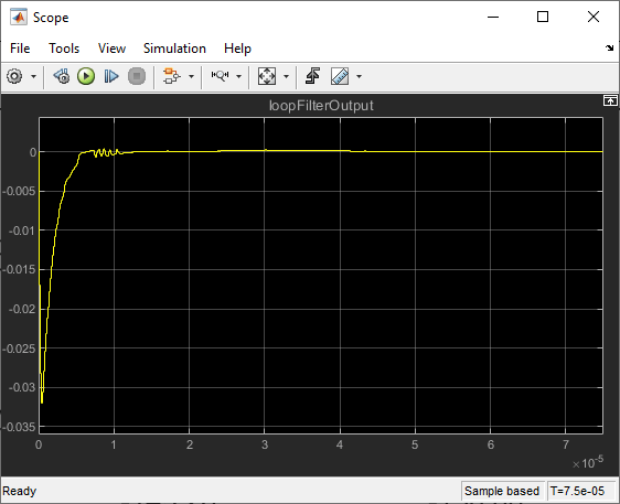
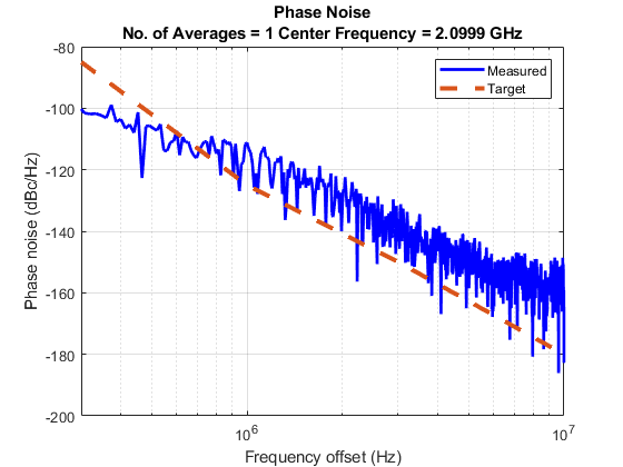
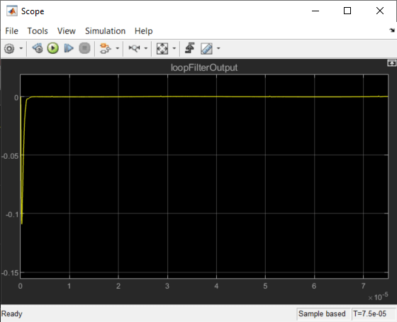
Simulate the model. The PLL Testbench block displays the PLL lock time and phase noise metrics. To plot and analyze the phase noise profile, in the PLL Testbench block parameters, on the Stimulus tab, select Plot phase noise. The measured lock time is 2.30 microseconds.
open_system([model,'/Scope'])
sim(model);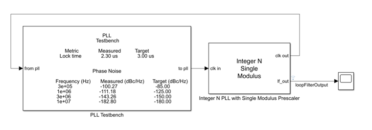
Define the PLL parameters needed to build the closed-loop system in MATLAB®.
PllKphi = 5e-3;     % Charge pump output current
PllKvco = 1e8;      % VCO sensitivity
PllN    = 70;       % Prescaler ratio

PllR2   = 88.3;     % Loop filter resistance for second-order response (ohms)
PllR3   = 253;      % Loop filter resistance for third-order response (ohms)
PllR4   = 642;      % Loop filter resistance for fourth-order response (ohms)
PllC1   = 8.13e-10; % Loop filter direct capacitance (F)
PllC2   = 1.48e-7;  % Loop filter capacitance for second-order response (F)
PllC3   = 1.59e-10; % Loop filter capacitance for third-order response (F)
PllC4   = 9.21e-11; % Loop filter capacitance for fourth-order response (F)
Build Custom Tunable System
To model the loop filter as a tunable element, first create tunable scalar real parameters (see realp) to represent each filter component. For each parameter, define the initial value and bounds. Also, specify whether the parameter is free to be tuned.
Use the current loop filter resistance and capacitance values as the initial numeric value of the tunable parameters.
% Resistances
R2 = realp('R2',PllR2);
R2.Minimum = 50;
R2.Maximum = 2000;
R2.Free = true;

R3 = realp('R3',PllR3);
R3.Minimum = 50;
R3.Maximum = 2000;
R3.Free = true;

R4 = realp('R4',PllR4);
R4.Minimum = 50;
R4.Maximum = 2000;
R4.Free = true;

% Capacitances
C1 = realp('C1',PllC1);
C1.Minimum = 1e-12;
C1.Maximum = 1e-7;
C1.Free = true;

C2 = realp('C2',PllC2);
C2.Minimum = 1e-12;
C2.Maximum = 1e-7;
C2.Free = true;

C3 = realp('C3',PllC3);
C3.Minimum = 1e-12;
C3.Maximum = 1e-7;
C3.Free = true;

C4 = realp('C4',PllC4);
C4.Minimum = 1e-12;
C4.Maximum = 1e-7;
C4.Free = true;
Using these tunable parameters, create a custom tunable model based on the loop filter transfer function equation specified in the More About section of the Loop Filter (Mixed-Signal Blockset) block reference page. loopFilterSys is a genss model parameterized by R2, R3, R4, C1, C2, C3, and C4.
A4 = C1*C2*C3*C4*R2*R3*R4;
A3 = C1*C2*R2*R3*(C3+C4)+C4*R4*(C2*C3*R3+C1*C3*R3+C1*C2*R2+C2*C3*R2);
A2 = C2*R2*(C1+C3+C4)+R3*(C1+C2)*(C3+C4)+C4*R4*(C1+C2+C3);
A1 = C1+C2+C3+C4;

loopFilterSys = tf([R2*C2, 1],[A4, A3, A2, A1, 0]);
Use the transfer function representations to define the fixed blocks in the architecture (charge pump, VCO, and prescaler), based on their respective frequency response characteristics [1].
chargePumpSys   = tf(PllKphi,1);       % Linearized as a static gain
vcoSys          = tf(PllKvco,[1 0]);   % Linearized as an integrator
prescalerSys    = tf(1/PllN,1);        % Linearized as a static gain
Define input and output names for each block. Connect the elements based on signal names (see connect) to create a tunable closed-loop system (see genss) representing the PLL architecture as shown.
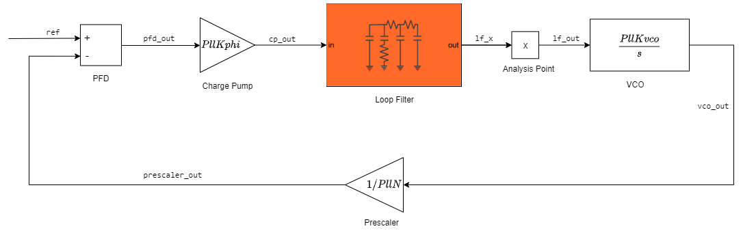
chargePumpSys.InputName = 'pfd_out';                % Charge pump (fixed block)
chargePumpSys.OutputName = 'cp_out';

loopFilterSys.InputName = 'cp_out';                 % Loop filter (tunable block)
loopFilterSys.OutputName = 'lf_x';

AP = AnalysisPoint('X');                            % Analysis point does not change the architecture of closed-loop system
AP.InputName = 'lf_x';
AP.OutputName = 'lf_out';

vcoSys.InputName = 'lf_out';                        % VCO (fixed block)
vcoSys.OutputName = 'vco_out';

prescalerSys.InputName = 'vco_out';                 % Prescaler (fixed block)
prescalerSys.OutputName = 'prescaler_out';

pfd = sumblk('pfd_out = ref - prescaler_out');      % Phase-frequency detector (sum block)

% Create a genss model for the closed-loop architecture
CL0 = connect(chargePumpSys,loopFilterSys,AP,vcoSys,prescalerSys,pfd,'ref','vco_out');
Loop-Shaping Design
Define the loop gain as a frequency-response data model by providing target gains for at least two decades below and two decades above the desired open-loop bandwidth. The desired roll-off is typically higher, which results in a higher attenuation of phase noise.
Specifying the appropriate target loop shape is the critical aspect of this design. The tunable compensator is a fourth-order system with a single integrator and a single zero, and the plant represents an integrator. The loop gains must be a feasible target for the open-loop structure.
For tuning the loop filter, create a tuning goal based on a target loop shape specifying the integral action, a 3 MHz crossover, and a roll-off requirement of 40 dB/decade. The goal is enforced for three decades below and above the desired open-loop bandwidth.
LoopGain = frd([100,10,1,1e-2,1e-4],2*pi*[1e4,1e5,3e6,3e7,3e8]);    % frd uses response data and corresponding frequencies in rad/s
LoopShapeGoal = TuningGoal.LoopShape('X',LoopGain);                 % Use AnalysisPoint as location where open-loop response shape is measured
LoopShapeGoal.Focus = 2*pi*[1e3, 1e9];                              % Enforce goal in frequency range (use rad/s)
LoopShapeGoal.Name = 'Loop Shape Goal';                             % Tuning goal name

MarginsGoal = TuningGoal.Margins('X',7.6,60);
MarginsGoal.Focus = [0 Inf];
MarginsGoal.Openings = {'X'};
MarginsGoal.Name = 'Margins Goal';
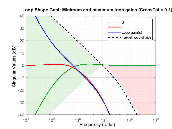
Observe the current open-loop shape of the PLL system with reference to the target loop shape. S represents the sensitivity function and T represents the complementary sensitivity function. By default, Control System Toolbox plots use rad/s as the frequency unit. For more information on how to change the frequency unit to Hz, see Specify Toolbox Settings for Linear Analysis Plots.
figure
viewGoal(LoopShapeGoal,CL0)
Use systune to tune the fixed-structure feedback loop. Doing so computes the resistance and capacitance values to meet the soft design goal based on the target loop shape. Run the tuning algorithm with five different initial value sets in addition to the initial values defined during the creation of the tunable scalar real parameters.
Options = systuneOptions();
Options.SoftTol = 1e-5;      % Relative tolerance for termination
Options.MinDecay = 1e-12;    % Minimum decay rate for closed-loop poles
Options.MaxRadius = 1e12;    % Maximum spectral radius for stabilized dynamics
Options.RandomStart = 5;     % Number of different random starting points

[CL,fSoft,gHard,Info] = systune(CL0,[LoopShapeGoal; MarginsGoal],[],Options);
Final: Soft = 2.85, Hard = -Inf, Iterations = 50
Final: Failed to enforce closed-loop stability (max Re(s) = 3.1e+04)
Final: Failed to enforce closed-loop stability (max Re(s) = 6.8e+04)
Final: Failed to enforce closed-loop stability (max Re(s) = 6.2e+04)
Final: Failed to enforce closed-loop stability (max Re(s) = 8e+04)
Final: Failed to enforce closed-loop stability (max Re(s) = 4.9e+04)
systune returns the tuned closed-loop system CL in generalized state-space form.
The algorithm fails to converge for the random initial values, and provides a feasible solution only when the current loop filter component values are chosen as the initial conditions. For tuning problems that are less complex, such as a third-order loop filter, the algorithm is less sensitive to initial conditions and randomized starts are an effective technique for exploring the parameter space and converging to a feasible solution.
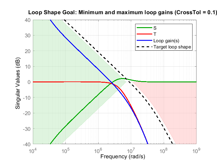
Examine the tuned open-loop shape with reference to the target loop shape. Observe that while the tuned loop shape does not meet the target, the open-loop bandwidth increases while the loop keeps the same high-frequency attenuation.
figure
viewGoal(LoopShapeGoal,CL)
Export Results to Simulink Model
Extract the tuned loop filter component values.
Rtuned = [getBlockValue(CL,'R2'),...
          getBlockValue(CL,'R3'),...
          getBlockValue(CL,'R4')];

Ctuned = [getBlockValue(CL,'C1'),...
          getBlockValue(CL,'C2'),...
          getBlockValue(CL,'C3'),...
          getBlockValue(CL,'C4')];
Write the tuned loop filter component values to the PLL block using the setLoopFilterValue helper function provided with the example.
blk = [model,'/Integer N PLL with Single Modulus Prescaler'];
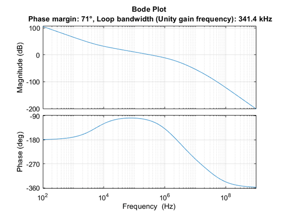
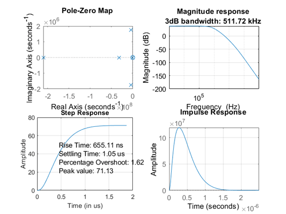
setLoopFilterValue(blk,Rtuned,Ctuned);Observe the Open Loop Analysis and Closed Loop Analysis plots from the Analysis tab in the Integer N PLL with Single Modulus Prescaler block parameters. The unity gain frequency and the 3-dB bandwidth show improvement and are now 341.4 kHz and 511.72 kHz, respectively, while the loop keeps the same phase noise profile.
Simulate the model and get the PLL Testbench measurements and loop filter output with the tuned components.
sim(model);

References
[1] Banerjee, Dean. PLL Performance, Simulation and Design. Indianapolis, IN: Dog Ear Publishing, 2006.
See Also
Topics
- Design and Evaluate Simple PLL Model (Mixed-Signal Blockset)
- Loop Shape and Stability Margin Specifications
- PLL Design and Verification Using Data Sheet Specifications (Mixed-Signal Blockset)