Parametric Fitting

R2026b

Parametric Fitting with Library Models

Parametric fitting involves finding coefficients (parameters) for one or more models that you fit to data. The data is assumed to be statistical in nature and is divided into two components:

data = deterministic component + random component

The deterministic component is given by a parametric model and the random component is often described as error associated with the data:

data = parametric model + error

The model is a function of the independent (predictor) variable and one or more coefficients. The error represents random variations in the data that follow a specific probability distribution (usually Gaussian). The variations can come from many different sources, but are always present at some level when you are dealing with measured data. Systematic variations can also exist, but they can lead to a fitted model that does not represent the data well.

The model coefficients often have physical significance. For example, suppose you collected data that corresponds to a single decay mode of a radioactive nuclide, and you want to estimate the half-life (T_1/2) of the decay. The law of radioactive decay states that the activity of a radioactive substance decays exponentially in time. Therefore, the model to use in the fit is given by

$$y=y_0{e}^{-\lambda t}$$

where y₀ is the number of nuclei at time t = 0, and λ is the decay constant. The data can be described by

$$\text{data}=y_0{e}^{-\lambda t}+\text{error}$$

Both y₀ and λ are coefficients that are estimated by the fit. Because T_1/2 = ln(2)/λ, the fitted value of the decay constant yields the fitted half-life. However, because the data contains some error, the deterministic component of the equation cannot be determined exactly from the data. Therefore, the coefficients and half-life calculation will have some uncertainty associated with them. If the uncertainty is acceptable, then you are done fitting the data. If the uncertainty is not acceptable, then you might have to take steps to reduce it either by collecting more data or by reducing measurement error and collecting new data and repeating the model fit.

With other problems where there is no theory to dictate a model, you might also modify the model by adding or removing terms, or substitute an entirely different model.

The Curve Fitting Toolbox™ parametric library models are described in the following sections.

Select Model Type

Select Model Type Interactively

Open the Curve Fitter app by entering curveFitter at the MATLAB^® command line. Alternatively, on the Apps tab, in the Math, Statistics and Optimization group, click Curve Fitter.

In the Curve Fitter app, go to the Fit Type section of the Curve Fitter tab. You can select a model type from the fit gallery. Click the arrow to open the gallery.

This table describes the models that you can fit for curves and surfaces.

Fit Group	Fit Type	Curves	Surfaces
Regression Models	Polynomial	Yes (up to degree 9)	Yes (up to degree 5)
	Exponential	Yes	No
	Logarithmic	Yes	No
	Fourier	Yes	No
	Gaussian	Yes	No
	Power	Yes	No
	Rational	Yes	No
	Sum of Sine	Yes	No
	Weibull	Yes	No
	Sigmoidal	Yes	No
Interpolation	Interpolant	Yes, with methods: Nearest neighbor Linear Cubic Shape-preserving (PCHIP)	Yes, with methods: Nearest neighbor Linear Natural neighbor Cubic Biharmonic (v4) Thin-plate spline
Smoothing	Smoothing Spline	Yes	No
	Lowess	No	Yes
Custom	Custom Equation	Yes	Yes
	Fit Custom Linear Models	Yes	No

The Results pane displays the model specifications, coefficient values, and goodness-of-fit statistics.

Tip

If your fit has problems, messages in the Results pane help you identify better settings.

The Curve Fitter app provides a selection of fit types and settings in the Fit Options pane that you can change to try to improve your fit. Try the defaults first, and then experiment with other settings. For more details on how to use the available fit options, see Coefficient Constraints: Specify Bounds and Optimized Start Points.

You can try a variety of settings for a single fit and you can create multiple fits to compare. When you create multiple fits in the Curve Fitter app, you can compare different fit types and settings side by side. For more information, see Create Multiple Fits in Curve Fitter App.

Select Model Type Programmatically

You can specify a library model name as a character vector or string scalar when you call the fit function. For example, you can specify a quadratic poly2 model:

f = fit(x,y,"poly2")

To view all available library model names, see List of Library Models for Curve and Surface Fitting.

You can also use the fittype function to construct a fittype object for a library model, and use the fittype as an input to the fit function.

Use the fitoptions function to find out what parameters you can set, for example:

fitoptions(poly2)

For examples, see the sections for each model type, listed in the table in Select Model Type Interactively. For details on all the functions for creating and analysing models, see Curve and Surface Fitting.

Center and Scale Data

Most fits in the Curve Fitter app provide the Center and scale option in the Fit Options pane. When you select this option, the app refits the model with the data centered and scaled.

To alleviate numerical problems like round-off errors with variables of large scales, normalize the input data (also known as predictor data). Center and scale generally improves the fit as it allows all variables to contribute to the fit similarly and results in less numerical instability. When you normalize inputs with this option, the values of the fitted coefficients change when compared to the original data, so the input data should not be normalized for cases where coefficients have a physical importance (e.g., eastings and northings for geographic data) or if the fitting is done to estimate coefficients.

The plots in the Curve Fitter app always use the original scale, regardless of the Center and scale status.

At the command line, to center and scale the data before fitting, use the fit function with Normalize="on" or create the options structure by using the fitoptions function with options.Normalize specified as "on". Then, use the fit function with the specified options.

options = fitoptions;
options.Normalize = "on";
options
options = 

  basefitoptions with properties:

    Normalize: 'on'
      Exclude: []
      Weights: []
       Method: 'None'

load census
f1 = fit(cdate,pop,"poly3",options)

Advanced Options

Curve Fitter App

In the Curve Fitter app, you can specify advanced fit options interactively in the Fit Options pane. All fits except Interpolant, Smoothing Spline, and Lowess have configurable advanced fit options. The available options depend on the fit you select (that is, linear, nonlinear, or nonparametric fit).

• Nonparametric fits (that is, Interpolant, Smoothing Spline, and Lowess fits) do not have Advanced Options.

• The options described below are available only for nonlinear models, unless specified otherwise.

The Fit Options pane for the single-term Exponential fit is shown here.

Fitting Method and Algorithm

• Method — Fit method

  The app automatically selects the Method value based on the fit you use. For linear and nonlinear fits, the Method value is LinearLeastSquares and NonlinearLeastSquares, respectively.

• Robust — Option for using the robust least-squares fitting method

  • Off — Do not use robust fitting (default).

  • LAR — Fit by minimizing the least absolute residuals (LAR).

  • Bisquare — Fit by minimizing the summed square of the residuals, and reduce the weight of outliers using bisquare weights. In most cases, this option is the best choice for robust fitting.

• Algorithm — Algorithm used for fitting

  • Trust-Region — This option is the default algorithm and can be used if you specify Lower or Upper coefficient constraints.

  • Levenberg-Marquardt — If the Trust-Region algorithm does not produce a reasonable fit, and you do not have coefficient constraints, try the Levenberg-Marquardt algorithm.

  • Interior-Point — If the previous algorithms do not result in a reasonable fit, try the Interior-Point algorithm. This algorithm must be selected for nonlinear fits if you have specified constraint points to fit through. The Optimization Toolbox™ is required to use this algorithm. Interior-Point can also be used if you specify coefficient constraints.

Finite Differencing Parameters

• DiffMinChange — Minimum change in coefficients for finite difference Jacobians. The default value is 10^-8.

• DiffMaxChange — Maximum change in coefficients for finite difference Jacobians. The default value is 0.1.

Note that DiffMinChange and DiffMaxChange apply to:

• Any nonlinear custom equation, that is, a nonlinear equation that you write

• Some of the nonlinear equations provided with Curve Fitting Toolbox

DiffMinChange and DiffMaxChange do not apply to any linear equations.

Fit Convergence Criteria

• MaxFunEvals — Maximum number of function (model) evaluations allowed. The default value is 600.

• MaxIter — Maximum number of fit iterations allowed. The default value is 400.

• TolFun — Termination tolerance used on stopping conditions involving the function (model) value. The default value is 10^-6.

• TolX — Termination tolerance used on stopping conditions involving the coefficients. The default value is 10^-6.

• TolCon — Tolerance for constraint points with a default value of 10^-6. This is the upper bound of the absolute numerical difference between the provided constraint point and the actual point the fit passes through, before a constraint violation occurs. If TolCon is satisfied, the solver still continues, unless it is halted for another reason. A solver does not halt simply because TolCon is satisfied. The Optimization Toolbox is required to specify this tolerance.

Command Line

Create the default fit options structure and set the option to center and scale the data before fitting:

options = fitoptions;
options.Normalize = 'on';
options
options = 

  basefitoptions with properties:

    Normalize: 'on'
      Exclude: []
      Weights: []
       Method: 'None'

Modifying the default fit options structure is useful when you want to set the Normalize, Exclude, or Weights fields, and then fit your data using the same options with different fitting methods. For example:

load census
f1 = fit(cdate,pop,"poly3",options);
f2 = fit(cdate,pop,"exp1",options);
f3 = fit(cdate,pop,"cubicspline",options);

Data-dependent fit options are returned in the third output argument of the fit function. For example, the smoothing parameter for smoothing spline is data-dependent:

[f,gof,out] = fit(cdate,pop,"smoothingspline");
smoothparam = out.p
smoothparam =
    0.0089

Use fit options to modify the default smoothing parameter for a new fit:

options = fitoptions("Method","SmoothingSpline","SmoothingParam",0.0098);
[f,gof,out] = fit(cdate,pop,"smoothingspline",options);

For more details on using fit options, see the fitoptions function.

Coefficient Constraints: Specify Bounds and Optimized Start Points

Constrain coefficients by specifying lower and upper bounds for the coefficients and provide starting points for the coefficients. At the command line, use the fit or fitoptions function with the Lower, Upper and StartPoint options. Start points can only be specified for nonlinear fittypes, as linear fittypes do not require start points. To learn more about the default constraints and optimized start points, see Optimized Starting Points and Default Constraints.

Coefficient Parameters

• Coefficients — Symbols for the unknown coefficients to be fitted

• StartPoint — The coefficient starting values. The default values depend on the fit. For Rational, Weibull, and custom fits, the default values are randomly selected within the range [0 1]. For all other nonlinear models in the Fit Type gallery, the starting values depend on the data set and are calculated heuristically.

• Lower — Lower bounds of the fitted coefficients. The app uses these bounds only with the Trust-Region and Interior-Point fitting algorithm. The default lower bounds for most fits in the Fit Options pane are -Inf, which indicates that the coefficients are unconstrained. However, a few models have finite default lower bounds. For example, for Gaussian fits, the app constrains the width parameter so that it cannot be less than 0.

• Upper — Upper bounds of the fitted coefficients. The app uses these bounds only with the Trust-Region and Interior-Point fitting algorithm. The default upper bounds for all fits in the Fit Options pane are Inf, which indicates that the coefficients are unconstrained.

For more information about these fit options, see the lsqcurvefit (Optimization Toolbox) function.

Optimized Starting Points and Default Constraints

The default coefficient starting points and constraints for fits in the Fit Type pane are shown in the following table. If the starting points are optimized, then they are calculated heuristically based on the current data set. Random starting points are defined on the interval [0 1] and linear models do not require starting points. If a model does not have constraints, the coefficients have neither a lower bound nor an upper bound. You can override the default starting points and constraints by providing your own values in the Fit Options pane.

Fit	Starting Points	Constraints
Linear Fitting	N/A	None
Custom Equation	Random	None
Exponential	Optimized	None
Logarithmic	N/A	None
Fourier	Optimized	None
Gaussian	Optimized	ci > 0
Polynomial	N/A	None
Power	Optimized	None
Rational	Random	None
Sum of Sine	Optimized	bi > 0
Weibull	Random	a, b > 0
Sigmoidal (with Model as 4-parameter logistic)	Optimized	x/c > 0

The Sum of Sine and Fourier fits are particularly sensitive to starting points, and the optimized values might be accurate for only a few terms in the associated equations.

Constraint Points to Fit Through (requires Optimization Toolbox)

Constrain regression fittypes to pass through specific points by adding Constraint Points in the Curve Fitter app or at the command line using the ConstraintPoints name-value argument. Nonparametric fits (that is, Interpolant, Smoothing Spline, and Lowess fits) do not accept constraint points.

Constraint points allow fitting the curve or surface through the origin, one or more data points, or any arbitrary coordinates.

• The number of constraint points cannot be greater than the number of coefficients in the fittype. For example, a one degree polynomial

  $$p_{1}x+p_2$$

  can be fit with maximum of two constraint points.

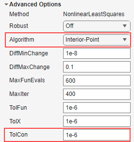
• The constraint tolerance can be specified by setting TolCon. It is the upper bound of the absolute numerical difference between the provided constraint point and the actual point the fit passes through, before considering it a constraint violation.

• The fitting algorithm must be Interior-Point when constraint points are provided for nonlinear fittypes i.e. when Method is NonlinearLeastSquares.

Tip

To debug a warning due to a constraint violation, repeat the workflow with constraint points at the command line with the Display name-value argument set to "iter".