Sequence Classification Using CNN-LSTM Network

This example shows how to create a 2-D CNN-LSTM network for speech classification tasks by combining a 2-D convolutional neural network (CNN) with a long short-term memory (LSTM) layer.

A CNN processes sequence data by applying sliding convolutional filters to the input. A CNN can learn features from both spatial and time dimensions. An LSTM network processes sequence data by looping over time steps and learning long-term dependencies between time steps. A CNN-LSTM network use convolutional and LSTM layers to learn from the training data.

To train a CNN-LSTM network with audio data, you extract auditory-based spectrograms from the raw audio data and then train the network using the spectrograms. This diagram illustrates the network application.

The example trains a 2-D CNN-LSTM network to recognize the emotion of spoken text by using the Berlin Database of Emotional Speech (Emo-DB) [1]. The emotions are text-independent, which means that the data contains no textual clues that indicate the emotion.

Download Data Set

Download the Emo-DB [1] data set. This dataset contains 535 utterances spoken by 10 actors labeled with one of these emotions: anger, boredom, disgust, anxiety/fear, happiness, sadness, or neutral.

dataFolder = fullfile(tempdir,"Emo-DB");
if ~datasetExists(dataFolder)
    url = "http://emodb.bilderbar.info/download/download.zip";
    disp("Downloading Emo-DB (40.5 MB) ...")
    unzip(url,dataFolder)
end

Create an audioDatastore (Audio Toolbox) object for the data.

location = fullfile(dataFolder,"wav");
ads = audioDatastore(location);

The file names encode the speaker ID, text spoken, emotion, and version. The emotion labels are encoded as:

• W — Anger

• L — Boredom

• E — Disgust

• A — Anxiety/Fear

• F — Happiness

• T — Sadness

• N — Neutral

Extract the emotion labels from the file names. The sixth character of the file name encodes the emotion labels.

filepaths = ads.Files;
[~,filenames] = fileparts(filepaths);
emotionLabels = extractBetween(filenames,6,6);

Replace the single-letter codes with the descriptive labels.

emotionCodeNames = ["W" "L" "E" "A" "F" "T" "N"];
emotionNames = ["Anger" "Boredom" "Disgust" "Anxiety/Fear" "Happiness" "Sadness" "Neutral"];
emotionLabels = replace(emotionLabels,emotionCodeNames,emotionNames);

Convert the labels to a categorical array.

emotionLabels = categorical(emotionLabels);

Set the Labels property of the audioDatastore object to emotionLabels.

ads.Labels = emotionLabels;

View the distribution of classes in a histogram.

figure
histogram(emotionLabels)
title("Class Distribution")
ylabel("Number of Observations")

Read a sample from the datastore, view the waveform in a plot, and listen to the sample.

[audio,info] = read(ads);
fs = info.SampleRate;
sound(audio,fs)

figure
plot((1:length(audio))/fs,audio)
title("Class: " + string(emotionLabels(1)))
xlabel("Time (s)")
ylabel("Amplitude")

Prepare Data for Training

Split the data into training, validation, and testing data. Use 70% of the data for training, 15% of the data for validation, and 15% of the data for testing.

[adsTrain,adsValidation,adsTest] = splitEachLabel(ads,0.70,0.15,0.15);

View the number of training observations.

numObservationsTrain = numel(adsTrain.Files)

numObservationsTrain = 371

Training a deep learning model usually requires many training observations to achieve a good fit. When you do not have much training data available, you can try to improve the fit of the network by artificially increasing the size of the training data using augmentations.

Create an audioDataAugmenter (Audio Toolbox) object:

• Specify 75 augmentations for each file. You can experiment with the number of augmentations for each file and compare the tradeoff between processing time and accuracy improvement.

• Set the probability of applying pitch shifting to 0.5.

• Set the probability of applying time shifting to 1 and set the range to [-0.3 0.3] seconds.

• Set the probability of adding noise to 1 and set the SNR range to [-20 40] dB.

numAugmentations = 75;

augmenter = audioDataAugmenter(NumAugmentations=numAugmentations, ...
    TimeStretchProbability=0, ...
    VolumeControlProbability=0, ...
    PitchShiftProbability=0.5, ...
    TimeShiftProbability=1, ...
    TimeShiftRange=[-0.3 0.3], ...
    AddNoiseProbability=1, ...
    SNRRange=[-20 40]);

Create a new folder to hold the augmented data.

agumentedDataFolder = fullfile(pwd,"augmentedData");
mkdir(agumentedDataFolder)

You can augment data as you input it to the network or augment the training data before training and save the augmented files to disk. In most cases, saving the results to disk reduces the overall training time and is useful when you want to experiment with different network architectures and training options.

Augment the training data by looping over the datastore and using the audio data augmenter. For each augmentation:

• Normalize the augmentation to have a maximum value of 1.

• Save the augmentation in a WAV file and append "_augK" to the file name, where K is the augmentation number.

To speed up the augmentation process, process the audio files in parallel using a parfor (Parallel Computing Toolbox) loop by splitting the audio datastore into smaller partitions and looping over the partitions in parallel. Using parfor requires a Parallel Computing Toolbox™ license. If you do not have a Parallel Computing Toolbox license, then the parfor loop runs in serial.

reset(ads)

numPartitions = 50;

augmentationTimer = tic;
parfor i = 1:numPartitions
    adsPart = partition(adsTrain,numPartitions,i);

    while hasdata(adsPart)
        [X,info] = read(adsPart);
        data = augment(augmenter,X,fs);

        [~,name] = fileparts(info.FileName);

        for n = 1:numAugmentations
            XAug = data.Audio{n};
            XAug = XAug/max(abs(XAug),[],"all");

            nameAug = name + "_aug" + string(n);

            filename = fullfile(agumentedDataFolder,nameAug + ".wav");
            audiowrite(filename,XAug,fs);
        end
    end
end
toc(augmentationTimer)

Elapsed time is 346.073556 seconds.

Create an audio datastore of the augmented data set.

augadsTrain = audioDatastore(agumentedDataFolder);

Because the file names of the augmented data and the original data differ only by a suffix, the labels of the augmented data are repeated elements of the original labels. Replicate the rows of the labels of the original datastore NumAugmentations times and assign them to the Labels property of the new datastore.

augadsTrain.Labels = repelem(adsTrain.Labels,augmenter.NumAugmentations,1);

Extract the features from the audio data using an audioFeatureExtractor (Audio Toolbox) object. Specify:

• A window length of 2048 samples

• A hop length of 512 samples

• A periodic Hamming window

• To extract the one-sided mel spectrum

windowLength = 2048;
hopLength = 512;

afe = audioFeatureExtractor( ...
    Window=hamming(windowLength,"periodic"), ...
    OverlapLength=(windowLength - hopLength), ...
    SampleRate=fs, ...
    melSpectrum=true);

Set the extractor parameters of the feature extractor. Set the number of mel bands to 128 and disable window normalization.

numBands = 128;
setExtractorParameters(afe,"melSpectrum", ...
    NumBands=numBands, ...
    WindowNormalization=false)

Extract the features and labels from the train, validation, and test datastores using the preprocessAudioData function, which is listed in the Preprocess Audio Data Function section of the example.

[featuresTrain,labelsTrain] = preprocessAudioData(augadsTrain,afe);
[featuresValidation,labelsValidation] = preprocessAudioData(adsValidation,afe);
[featuresTest,labelsTest] = preprocessAudioData(adsTest,afe);

Plot the waveforms and auditory spectrograms of a few training samples.

numPlots = 3;
idx = randperm(numel(augadsTrain.Files),numPlots);
f = figure;
f.Position(3) = 2*f.Position(3);

tiledlayout(2,numPlots,TileIndexing="columnmajor")

for ii = 1:numPlots
    [X,fs] = audioread(augadsTrain.Files{idx(ii)});

    nexttile
    plot(X)
    axis tight

    title(augadsTrain.Labels(idx(ii)))
    xlabel("Time")
    ylabel("Amplitude")

    nexttile
    spect = permute(featuresTrain{idx(ii)}(:,1,:), [1 3 2]);
    pcolor(spect)
    shading flat

    xlabel("Time")
    ylabel("Frequency")
end

View the sizes of the first few observations. The observations are sequences of samples with one spatial dimension. The observations have size numBands-by-1-by-numTimeSteps, where numBands corresponds to the spatial dimension of the data and numTimeSteps corresponds to the time dimension of the data.

featuresTrain(1:10)

ans=10×1 cell array
    {128×1×56 double}
    {128×1×56 double}
    {128×1×56 double}
    {128×1×56 double}
    {128×1×56 double}
    {128×1×56 double}
    {128×1×56 double}
    {128×1×56 double}
    {128×1×56 double}
    {128×1×56 double}

To ensure that the network supports the training data, you can use the MinLength option of the sequence input layer to check that sequences can flow through the network. Calculate the length of the shortest sequence to pass to the input layer.

sequenceLengths = zeros(1,numObservationsTrain);
for n = 1:numObservationsTrain
    sequenceLengths(n) = size(featuresTrain{n},3);
end
minLength = min(sequenceLengths)

minLength = 41

Define 2-D CNN LSTM Architecture

Define the 2-D CNN LSTM network based on [2] that predicts class labels of sequences.

• For sequence input, specify a sequence input layer with an input size matching the input data. To ensure that the network supports the training data, set the MinLength option to the length of the shortest sequence in the training data.

• To learn spatial relations in the 1-D image sequences, use a 2-D CNN architecture with four repeating blocks of convolutional, batch normalization, ReLU, and max pooling layers. Specify an increasing number of filters for the third and fourth convolutional layers.

• To learn long-term dependencies in the 1-D image sequences, include an LSTM layer with 256 hidden units. To map the sequences to a single value for prediction, output only the last time step by setting the OutputMode option to "last".

• For classification, include a fully connected layer with a size equal to the number of classes. To convert the output to vectors of probabilities, include a softmax layer.

• Include a classification layer.

filterSize = 3;
numFilters = 64;
numHiddenUnits = 256;

inputSize = [numBands 1];
numClasses = numel(categories(emotionLabels));

layers = [
    sequenceInputLayer(inputSize,MinLength=minLength)

    convolution2dLayer(filterSize,numFilters,Padding="same")
    batchNormalizationLayer
    reluLayer
    maxPooling2dLayer(2,Stride=2)

    convolution2dLayer(filterSize,numFilters,Padding="same")
    batchNormalizationLayer
    reluLayer
    maxPooling2dLayer([4 2],Stride=[4 2])

    convolution2dLayer(filterSize,2*numFilters,Padding="same")
    batchNormalizationLayer
    reluLayer
    maxPooling2dLayer([4 2],Stride=[4 2])

    convolution2dLayer(filterSize,2*numFilters,Padding="same")
    batchNormalizationLayer
    reluLayer
    maxPooling2dLayer([4 2],Stride=[4 2])

    flattenLayer
    lstmLayer(numHiddenUnits,OutputMode="last")

    fullyConnectedLayer(numClasses)

    softmaxLayer
    classificationLayer];

Specify Training Options

Specify the training options using the trainingOptions function:

• Train a network using the Adam solver with a mini-batch size of 32 for three epochs.

• Train with an initial learning rate of 0.005 and reduce the learning rate in a piecewise manner after two epochs.

• To avoid overfitting the training data, specify an L2 regularization term with a value of 0.0005.

• To prevent padding values affecting the last time steps of the sequences that the LSTM layer outputs, left-pad the training sequences.

• Shuffle the data every epoch.

• Validate the training progress using the validation data once per epoch.

• Display the training progress in a plot and suppress verbose output.

• Train on a GPU if one is available. Using a GPU requires a Parallel Computing Toolbox license and a supported GPU device. For information on supported devices, see GPU Computing Requirements (Parallel Computing Toolbox).

miniBatchSize = 32;

options = trainingOptions("adam", ...
    MaxEpochs=3, ...
    MiniBatchSize=miniBatchSize, ...
    InitialLearnRate=0.005, ...
    LearnRateDropPeriod=2, ...
    LearnRateSchedule="piecewise", ...
    L2Regularization=5e-4, ...
    SequencePaddingDirection="left", ...
    Shuffle="every-epoch", ...
    ValidationFrequency=floor(numel(featuresTrain)/miniBatchSize), ...
    ValidationData={featuresValidation,labelsValidation}, ...
    Verbose=false, ...
    Plots="training-progress");

Train Network

Train the network using the trainNetwork function. If you do not have a GPU, then training the network can take a long time to run.

net = trainNetwork(featuresTrain,labelsTrain,layers,options);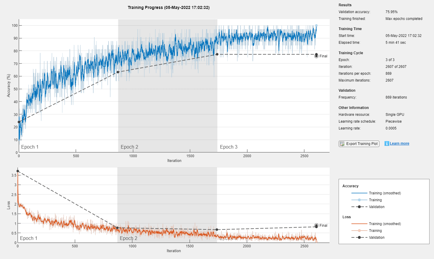

Test Network

Test the classification accuracy of the model by comparing the predictions on the held-out test set with the true labels for each test observation.

Classify the test data using the trained network.

labelsPred = classify(net,featuresTest, ...
    MiniBatchSize=miniBatchSize, ...
    SequencePaddingDirection="left");

Visualize the predictions in a confusion matrix.

figure
confusionchart(labelsTest,labelsPred)

Evaluate the classification accuracy by comparing the predictions to the test labels.

accuracy = mean(labelsPred == labelsTest)

accuracy = 0.6329

Supporting Functions

Preprocess Audio Data Function

The preprocessAudioData function extracts the features and labels from the audio datastore ads using the audio feature extractor afe. The function transforms the data using the extractFeatures function, listed in the Extract Features Function section of the example, as a datastore transform function. To process the data, the function creates the transformed datastore and reads all the data using the readall function. To read the data in parallel, the function sets the UseParallel option of the readall function. Reading in parallel requires a Parallel Computing Toolbox license. To check if you can use a parallel pool for reading the data, the function uses the canUseParallelPool function.

function [features,labels] = preprocessAudioData(ads,afe)

% Transform datastore.
tds = transform(ads,@(X) extractFeatures(X,afe));

% Read all data.
tf = canUseParallelPool;
features = readall(tds,UseParallel=tf);

% Extract labels.
labels = ads.Labels;

end

Extract Features Function

The extractFeatures function extracts features from the audio data X using the audio feature extractor afe. The function computes the logarithm of the extracted features and permutes the data to have size numBands-by-1-by-numTimeSteps for training.

function features = extractFeatures(X,afe)

features = log(extract(afe,X) + eps);
features = permute(features, [2 3 1]);
features = {features};

end

References

[1] Burkhardt, Felix, A. Paeschke, M. Rolfes, Walter F. Sendlmeier, and Benjamin Weiss. “A Database of German Emotional Speech.” In Interspeech 2005, 1517–20. ISCA, 2005. https://doi.org/10.21437/Interspeech.2005-446.

[2] Zhao, Jianfeng, Xia Mao, and Lijiang Chen. “Speech Emotion Recognition Using Deep 1D & 2D CNN LSTM Networks.” Biomedical Signal Processing and Control 47 (January 2019): 312–23. https://doi.org/10.1016/j.bspc.2018.08.035.