Discrete-Time Markov Chains
What Are Discrete-Time Markov Chains?
Consider a stochastic process taking values in a state space. A Markov process evolves in a manner that is independent of the path that leads to the current state. That is, the current state contains all the information necessary to forecast the conditional probabilities of future paths. This characteristic is called the Markov property. Although a Markov process is a specific type of stochastic process, it is widely used in modeling changes of state. The specificity of a Markov process leads to a theory that is relatively complete.
Markov processes can be restricted in various ways, leading to progressively more concise mathematical formulations. The following conditions are examples of restrictions.
The state space can be restricted to a discrete set. This characteristic is indicative of a Markov chain. The transition probabilities of the Markov property “link” each state in the chain to the next.
If the state space is finite, the chain is finite-state.
If the process evolves in discrete time steps, the chain is discrete-time.
If the Markov property is time-independent, the chain is homogeneous.
Econometrics Toolbox™ includes the dtmc model
object representing a finite-state, discrete-time, homogeneous Markov chain. Even
with restrictions, the dtmc object has great applicability. It is
robust enough to serve in many modeling scenarios in econometrics, and the
mathematical theory is well suited for the matrix algebra of MATLAB®.
Finite-state Markov chains have a dual theory: one in matrix analysis and one in
discrete graphs. Object functions of the dtmc object highlight this
duality. The functions allow you to move back and forth between numerical and
graphical representations. You can work with the tools that are best suited for
particular aspects of an investigation. In particular, traditional eigenvalue
methods for determining the structure of a transition matrix are paired with
visualizations for tracing the evolution of a chain through its associated
digraph.
A key feature of any Markov chain is its limiting behavior. This feature is
especially important in econometric applications, where the forecast performance of
a model depends on whether its stochastic component has a well-defined distribution,
asymptotically. Object functions of the dtmc object allow you to
investigate transient and steady-state behavior of a chain and the properties that
produce a unique limit. Other functions compute the limiting distribution and
estimate rates of convergence, or mixing times.
Simulation of the underlying stochastic process of a suitable Markov chain is
fundamental to application. Simulation can take the form of generating a random
sequence of state transitions from an initial state or from the time evolution of an
entire distribution of states. Simulation allows you to determine statistical
characteristics of a chain that might not be evident from its specification or the
theory. In econometrics, Markov chains become components of larger regime-switching
models, where they represent shifts in the economic environment. The
dtmc object includes functions for simulating and visualizing
the time evolution of Markov chains.
Discrete-Time Markov Chain Theory
Any finite-state, discrete-time, homogeneous Markov chain can be represented,
mathematically, by either its n-by-n
transition matrix P, where n is the number of
states, or its directed graph D. Although the two representations
are equivalent—analysis performed in one domain leads to equivalent results in the
other—there are considerable differences in both the conception of analytic
questions and the resulting algorithmic solutions. This dichotomy is best
illustrated by comparing the development of the theory in [7], for example,
with the developments in [6] and [9]. Or, using
MATLAB, the dichotomy can be illustrated by comparing the algorithms based on
the graph object and its functions with the
core functionality in matrix analysis.
The complete graph for a finite-state process has edges and transition probabilities between every node i and every other node j. Nodes represent states in the Markov chain. In D, if the matrix entry Pij is 0, then the edge connecting states i and j is removed. Therefore, D shows only the feasible transitions among states. Also, D can include self-loops indicating nonzero probabilities Pii of transition from state i back to itself. Self-transition probabilities are known as state inertia or persistence.
In D, a walk between states i and j is a sequence of connected states that begins at i and ends at j, and has a length of at least two. A path is a walk without repeated states. A circuit is a walk in which i = j, but no other repeated states are present.
State j is reachable, or accessible, from state i, denoted , if there is a walk from i to j. The states communicate, denoted , if each is reachable from the other. Communication is an equivalence relation on the state space, partitioning it into communicating classes. In graph theory, states that communicate are called strongly connected components. For the Markov processes, important properties of individual states are shared by all other states in a communicating class, and so become properties of the class itself. These properties include:
Recurrence — The property of being reachable from all states that are reachable. This property is equivalent to an asymptotic probability of return equal to 1. Every chain has at least one recurrent class.
Transience — The property of not being recurrent, that is, the possibility of accessing states from which there is no return. This property is equivalent to an asymptotic probability of return equal to 0. Classes with transience have no effect on asymptotic behavior.
Periodicity — The property of cycling among multiple subclasses within a class and retaining some memory of the initial state. The period of a state is the greatest common divisor of the lengths of all circuits containing the state. States or classes with period 1 are aperiodic. Self-loops on states ensure aperiodicity and form the basis for lazy chains.
An important property of a chain as a whole is irreducibility. A chain is irreducible if the chain consists of a single communicating class. State or class properties become properties of the entire chain, which simplifies the description and analysis. A generalization is a unichain, which is a chain consisting of a single recurrent class and any number of transient classes. Important analyses related to asymptotics can be focused on the recurrent class.
A condensed graph, which is formed by consolidating the states of each class into a single supernode, simplifies visual understanding of the overall structure. In this figure, the single directed edge between supernodes C1 and C2 corresponds to the unique transition direction between the classes.
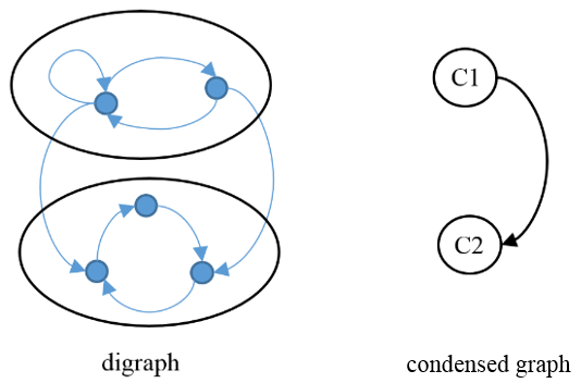
The condensed graph shows that C1 is transient and C2 is recurrent. The outdegree of C1 is positive, which implies transience. Because C1 contains a self-loop, it is aperiodic. C2 is periodic with a period of 3. The single states in the three-cycle of C2 are, in a more general periodic class, communicating subclasses. The chain is a reducible unichain. Imagine a directed edge from C2 to C1. In that case, C1 and C2 are communicating classes, and they collapse into a single node.
Ergodicity, a desirable property, combines irreducibility with aperiodicity and guarantees uniform limiting behavior. Because irreducibility is inherently a chain property, not a class property, ergodicity is a chain property as well. When used with unichains, ergodicity means that the unique recurrent class is ergodic.
With these definitions, it is possible to summarize the fundamental existence and uniqueness theorems related to 1-by-n stationary distributions , where .
If P is right stochastic, then always has a probability vector solution. Because every row of P sums to one, P has a right eigenvector with an eigenvalue of one. Specifically, e = 1n, an n-by-1 vector of ones. So, P also has a left eigenvector with an eigenvalue of one. As a consequence of the Perron-Frobenius Theorem, is nonnegative and can be normalized to produce a probability vector.
is unique if and only if P represents a unichain. In general, if a chain contains k recurrent classes, π* = π*P has k linearly independent solutions. In this case, Pm converges as , but the rows are not identical.
Every initial distribution π0 converges to if and only if P represents an ergodic unichain. In this case, is a limiting distribution.
The Perron-Frobenius Theorem is a collection of results related to the eigenvalues of nonnegative, irreducible matrices. Applied to Markov chains, the results can be summarized as follows. For a finite-state unichain, P has a single eigenvalue λ1 = 1 (the Perron-Frobenius eigenvalue) with an accompanying nonnegative left eigenvector (which can be normalized to a probability vector) and a right eigenvector e = 1n. The other eigenvalues λi satisfy , i = 2,…,n. If the unichain or the sole recurrent class of the unichain is aperiodic, then the inequality is strict. When there is periodicity of period k, there are k eigenvalues on the unit circle at the k roots of unity. If the unichain is ergodic, then Pm converges asymptotically to as . The error goes to 0 at least as fast as , where λs is the eigenvalue of second largest magnitude and q is the multiplicity of λs.
The rate of convergence to depends on the second largest eigenvalue modulus (SLEM) . The rate can be expressed in terms of the spectral gap, which is . Large gaps yield faster convergence. The mixing time is a characteristic time for the deviation from equilibrium, in total variation distance. Because convergence is exponential, a mixing time for the decay by a factor of e1 is
Given the convergence theorems, mixing times should be viewed in the context of ergodic unichains.
Related theorems in the theory of nonnegative, irreducible matrices give convenient characterizations of the two crucial properties for uniform convergence: reducibility and ergodicity. Suppose Z is the indicator or zero pattern of P, that is, the matrix with ones in place of nonzero entries in P. Then, P is irreducible if and only if all entries of are positive. Wielandt’s theorem [11] states that P is ergodic if and only if all entries of Pm are positive for .
The Perron-Frobenius Theorem and related results are nonconstructive for the stationary distribution . There are several approaches for computing the unique limiting distribution of an ergodic chain.
Define the return time Tii to state i as the minimum number of steps to return to state i after starting in state i. Also, define mean return time τii as the expected value of Tii. Then, . This result has much intuitive content. Individual mean mixing times can be estimated by Monte Carlo simulation. However, the overhead of simulation and the difficulties of assessing convergence, make Monte Carlo simulation impractical as a general method.
Because Pm approaches a matrix with all rows equal to as , any row of a “high power” of P approximates π*. Although this method is straightforward, it involves choosing a convergence tolerance and an appropriately large m for each P. In general, the complications of mixing time analysis also make this computation impractical.
The linear system can be augmented with the constraint , in the form , where 1n-by-n is an n-by-n matrix of ones. Using the constraint, this system becomes
The system can be solved efficiently with the MATLAB backslash operator and is numerically stable because ergodic P cannot have ones along the main diagonal (otherwise P would be reducible). This method is recommended in [5].
Because is the unique left eigenvector associated with the Perron-Frobenius eigenvalue of P, sorting eigenvalues and corresponding eigenvectors identifies . Because the constraint is not part of the eigenvalue problem, requires normalization. This method uses the robust numerics of the MATLAB
eigsfunction, and is the approach implemented by theasymptoticsobject function of adtmcobject.
For any Markov chain, a finite-step analysis can suggest its asymptotic properties and mixing rate. A finite-step analysis includes the computation of these quantities:
The hitting probability is the probability of ever hitting any state in the subset of states A (target), beginning from state i in the chain. Categorically, hitting probabilities show which states are reachable from other states; > 0 means the target A is reachable from state i. If = 0, target A is unreachable from state i, meaning state i is remote for the target. If A forms a recurrent class, is the absorption probability.
The expected first hitting time is the long-run average number of time steps required to reach A for the first time, beginning from state i. = ∞ means one of the following alternatives:
The starting state i is remote for target A.
The starting state i is remote-reachable for target A; that is, > 0 and > 0, where B is a recurrent class not containing any states in A.
If A forms a recurrent class, is the expected absorption time.
A vector of the hitting probabilities or expected first hitting times for a target, beginning from each state in a Markov chain, suggests the mixing rate of the chain.
References
[1] Diebold, F.X., and G.D. Rudebusch. Business Cycles: Durations, Dynamics, and Forecasting. Princeton, NJ: Princeton University Press, 1999.
[2] Gallager, R.G. Stochastic Processes: Theory for Applications. Cambridge, UK: Cambridge University Press, 2013.
[3] Gilks, W. R., S. Richardson, and D.J. Spiegelhalter. Markov Chain Monte Carlo in Practice. Boca Raton: Chapman & Hall/CRC, 1996.
[4] Haggstrom, O. Finite Markov Chains and Algorithmic Applications. Cambridge, UK: Cambridge University Press, 2002.
[5] Hamilton, James D. Time Series Analysis. Princeton, NJ: Princeton University Press, 1994.
[6] Horn, R., and C. R. Johnson. Matrix Analysis. Cambridge, UK: Cambridge University Press, 1985.
[7] Jarvis, J. P., and D. R. Shier. "Graph-Theoretic Analysis of Finite Markov Chains." In Applied Mathematical Modeling: A Multidisciplinary Approach. Boca Raton: CRC Press, 2000.
[8] Maddala, G. S., and I. M. Kim. Unit Roots, Cointegration, and Structural Change. Cambridge, UK: Cambridge University Press, 1998.
[9] Montgomery, J. Mathematical Models of Social Systems. Unpublished manuscript. Department of Sociology, University of Wisconsin-Madison, 2016.
[10] Norris, J. R. Markov Chains. Cambridge, UK: Cambridge University Press, 1997.
[11] Wielandt, H. Topics in the Analytic Theory of Matrices. Lecture notes prepared by R. Mayer. Department of Mathematics, University of Wisconsin-Madison, 1967.
See Also
Objects
Functions
eigs|asymptotics|isergodic|isreducible|classify|lazy|graphplot|eigplot|mcmix