dtmc
Create discrete-time Markov chain
Description
dtmc creates a discrete-time, finite-state, time-homogeneous Markov chain from a specified state transition matrix.
After creating a dtmc object, you can analyze the structure and
evolution of the Markov chain, and visualize the Markov chain in various ways, by using
the object
functions. Also, you can use a dtmc object to specify the
switching mechanism of a Markov-switching dynamic regression model (msVAR).
To create a switching mechanism, governed by threshold transitions and threshold
variable data, for a threshold-switching dynamic regression model, see threshold and
tsVAR.
Creation
Description
mc = dtmc(P)mc specified by the state transition matrix P.
mc = dtmc(P,'StateNames',stateNames)stateNames to the
states.
Input Arguments
Properties
Object Functions
dtmc objects require a fully specified transition matrix P.
Examples
Consider this theoretical, right-stochastic transition matrix of a stochastic process.
Element is the probability that the process transitions to state j at time t + 1 given that it is in state i at time t, for all t.
Create the Markov chain that is characterized by the transition matrix P.
P = [0.5 0.5 0 0; 0.5 0 0.5 0; 0 0 0 1; 0 0 1 0];
mc = dtmc(P);
mc is a dtmc object that represents the Markov chain.
Display the number of states in the Markov chain.
numstates = mc.NumStates
numstates =
4
Plot a directed graph of the Markov chain.
figure;
graphplot(mc);
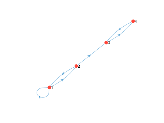
Observe that states 3 and 4 form an absorbing class, while states 1 and 2 are transient.
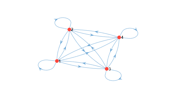
Consider this transition matrix in which element is the observed number of times state i transitions to state j.
For example, implies that state 3 transitions to state 2 seven times.
P = [16 2  3  13;
     5  11 10 8;
     9  7  6  12;
     4  14 15 1];
Create the Markov chain that is characterized by the transition matrix P.
mc = dtmc(P);
Display the normalized transition matrix stored in mc. Verify that the elements within rows sum to 1 for all rows.
mc.P
ans = 4×4

    0.4706    0.0588    0.0882    0.3824
    0.1471    0.3235    0.2941    0.2353
    0.2647    0.2059    0.1765    0.3529
    0.1176    0.4118    0.4412    0.0294
sum(mc.P,2)
ans = 4×1

     1
     1
     1
     1
Plot a directed graph of the Markov chain.
figure;
graphplot(mc);
Consider the two-state business cycle of the US real gross national product (GNP) in [3] p. 697. At time t, real GNP can be in a state of expansion or contraction. Suppose that the following statements are true during the sample period.
If real GNP is expanding at time t, then the probability that it will continue in an expansion state at time t + 1 is .
If real GNP is contracting at time t, then the probability that it will continue in a contraction state at time t + 1 is .
Create the transition matrix for the model.
p11 = 0.90;
p22 = 0.75;

P = [p11 (1 - p11); (1 - p22) p22];
Create the Markov chain that is characterized by the transition matrix P. Label the two states.
mc = dtmc(P,'StateNames',["Expansion" "Contraction"])
mc =
  dtmc with properties:

             P: [2×2 double]
    StateNames: ["Expansion"    "Contraction"]
     NumStates: 2
Plot a directed graph of the Markov chain. Indicate the probability of transition by using edge colors.
figure;
graphplot(mc,'ColorEdges',true);
To help you explore the dtmc object functions, mcmix creates a Markov chain from a random transition matrix using only a specified number of states.
Create a five-state Markov chain from a random transition matrix.
rng(1); % For reproducibility
mc = mcmix(5)
mc =
dtmc with properties:
P: [5×5 double]
StateNames: ["1" "2" "3" "4" "5"]
NumStates: 5
mc is a dtmc object.
Plot the eigenvalues of the transition matrix on the complex plane.
figure;
eigplot(mc)
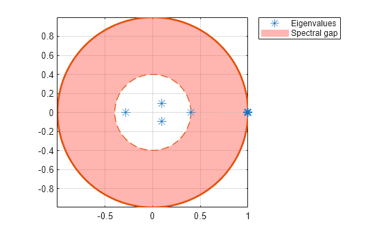
This spectrum determines structural properties of the Markov chain, such as periodicity and mixing rate.
Consider a Markov-switching autoregression (msVAR) model for the US GDP containing four economic regimes: depression, recession, stagnation, and expansion. To estimate the transition probabilities of the switching mechanism, you must supply a dtmc model with an unknown transition matrix entries to the msVAR framework.
Create a 4-regime Markov chain with an unknown transition matrix (all NaN entries). Specify the regime names.
P = nan(4);
statenames = ["Depression" "Recession" ...
    "Stagnation" "Expansion"];

mcUnknown = dtmc(P,'StateNames',statenames)
mcUnknown =
  dtmc with properties:

             P: [4×4 double]
    StateNames: ["Depression"    "Recession"    "Stagnation"    "Expansion"]
     NumStates: 4
mcUnknown.P
ans = 4×4

   NaN   NaN   NaN   NaN
   NaN   NaN   NaN   NaN
   NaN   NaN   NaN   NaN
   NaN   NaN   NaN   NaN
Suppose economic theory states that the US economy never transitions to an expansion from a recession or depression. Create a 4-regime Markov chain with a partially known transition matrix representing the situation.
P(1,4) = 0;
P(2,4) = 0;

mcPartial = dtmc(P,'StateNames',statenames)
mcPartial =
dtmc with properties:
P: [4×4 double]
StateNames: ["Depression" "Recession" "Stagnation" "Expansion"]
NumStates: 4
mcPartial.P
ans = 4×4

   NaN   NaN   NaN     0
   NaN   NaN   NaN     0
   NaN   NaN   NaN   NaN
   NaN   NaN   NaN   NaN
The estimate function of msVAR treats the known elements of mcPartial.P as equality constraints during optimization.
For more details on Markov-switching dynamic regression models, see msVAR.
Alternatives
You also can create a Markov chain object using mcmix.
References
[1] Gallager, R.G. Stochastic Processes: Theory for Applications. Cambridge, UK: Cambridge University Press, 2013.
[2] Haggstrom, O. Finite Markov Chains and Algorithmic Applications. Cambridge, UK: Cambridge University Press, 2002.
[3] Hamilton, James D. Time Series Analysis. Princeton, NJ: Princeton University Press, 1994.
[4] Norris, J. R. Markov Chains. Cambridge, UK: Cambridge University Press, 1997.
Version History
Introduced in R2017b