Main Content

optSensByHestonFFT

Option price and sensitivities by Heston model using FFT and FRFT

Description

example

[PriceSens,StrikeOut] = optSensByHestonFFT(Rate,AssetPrice,Settle,Maturity,OptSpec,Strike,V0,ThetaV,Kappa,SigmaV,RhoSV) computes vanilla European option price and sensitivities by Heston model, using Carr-Madan FFT and Chourdakis FRFT methods.

Note

Alternatively, you can use the Vanilla object to calculate price or sensitivities for vanilla options. For more information, see Get Started with Workflows Using Object-Based Framework for Pricing Financial Instruments.

example

[PriceSens,StrikeOut] = optSensByHestonFFT(___,Name,Value) adds optional name-value pair arguments.

Examples

collapse all

Use optSensByHestonFFT to calibrate the FFT strike grid for sensitivities, compute option sensitivities, and plot option sensitivity surfaces.

Define Option Variables and Heston Model Parameters

AssetPrice = 80;
Rate = 0.03;
DividendYield = 0.02;
OptSpec = 'call';

V0 = 0.04;
ThetaV = 0.05;
Kappa = 1.0;
SigmaV = 0.2;
RhoSV = -0.7;

Compute the Option Sensitivities for the Entire FFT (or FRFT) Strike Grid, Without Specifying "Strike"

Compute option sensitivities and also output the corresponding strikes. If the Strike input is empty ( [] ), option sensitivities will be computed on the entire FFT (or FRFT) strike grid. The FFT (or FRFT) strike grid is determined as exp(log-strike grid), where each column of the log-strike grid has NumFFT points with LogStrikeStep spacing that are roughly centered around each element of log(AssetPrice). The default value for NumFFT is 2^12. In addition to the sensitivities in the first output, the optional last output contains the corresponding strikes.

Settle = datetime(2017,6,29);
Maturity = datemnth(Settle, 6);
Strike = []; % Strike is not specified (will use the entire FFT strike grid)

% Compute option sensitivities for the entire FFT strike grid
[Delta, Kout] = optSensByHestonFFT(Rate, AssetPrice, Settle, Maturity, OptSpec, Strike, ...
    V0, ThetaV, Kappa, SigmaV, RhoSV, 'DividendYield', DividendYield, 'OutSpec', "delta");

% Show the lowest and highest strike values on the FFT strike grid
format
MinStrike = Kout(1) % Lowest possible strike in the current FFT strike grid
MinStrike = 2.9205e-135
MaxStrike = Kout(end) % Highest possible strike in the current FFT strike grid
MaxStrike = 1.8798e+138
% Show a subset of the strikes and corresponding option sensitivities
Range = (2046:2052);
[Kout(Range) Delta(Range)]
ans = 7×2

   50.4929    0.9866
   58.8640    0.9671
   68.6231    0.8724
   80.0000    0.5775
   93.2631    0.1545
  108.7251    0.0059
  126.7505    0.0000

Change the Number of FFT (or FRFT) Points, and Compare With optSensByHestonNI

Try a different number of FFT (or FRFT) points, and compare the results with numerical integration. Unlike optSensByHestonFFT, which uses FFT (or FRFT) techniques for fast computation across the whole range of strikes, the optSensByHestonNI function uses direct numerical integration and it is typically slower, especially for multiple strikes. However, the values computed by optSensByHestonNI can serve as a benchmark for adjusting the settings for optSensByHestonFFT.

% Try a smaller number of FFT points 
% (e.g. for faster performance or smaller memory footprint)
NumFFT = 2^10; % Smaller than the default value of 2^12 
Strike = []; % Strike is not specified (will use the entire FFT strike grid)
[Delta, Kout] = optSensByHestonFFT(Rate, AssetPrice, Settle, Maturity, OptSpec, Strike, ...
    V0, ThetaV, Kappa, SigmaV, RhoSV, 'DividendYield', DividendYield, ...
    'OutSpec', "delta", 'NumFFT', NumFFT);

% Compare with numerical integration method
Range = (510:516);
Strike = Kout(Range);
DeltaFFT = Delta(Range);
DeltaNI = optSensByHestonNI(Rate, AssetPrice, Settle, Maturity, OptSpec, Strike, ...
    V0, ThetaV, Kappa, SigmaV, RhoSV, 'DividendYield', DividendYield, 'OutSpec', "delta");
Error = abs(DeltaFFT-DeltaNI);
table(Strike, DeltaFFT, DeltaNI, Error)
ans=7×4 table
    Strike     DeltaFFT      DeltaNI        Error   
    ______    __________    __________    __________

    12.696       0.90066       0.99002       0.08936
    23.449       0.93635       0.99002      0.053677
    43.312       0.94796        0.9896      0.041645
        80       0.53274       0.57747      0.044733
    147.76     0.0032769      2.45e-08     0.0032769
    272.93    0.00098029    -1.399e-10    0.00098029
    504.11    0.00028151    5.2868e-10    0.00028151

Make Further Adjustments to FFT (or FRFT)

If the values in the output DeltaFFT are significantly different from those in DeltaNI, try making adjustments to optSensByHestonFFT settings, such as CharacteristicFcnStep, LogStrikeStep, NumFFT, DampingFactor, and so on. Note that if (LogStrikeStep * CharacteristicFcnStep) is 2*pi/ NumFFT, FFT is used. Otherwise, FRFT is used.

Strike = []; % Strike is not specified (will use the entire FFT or FRFT strike grid)
[Delta, Kout] = optSensByHestonFFT(Rate, AssetPrice, Settle, Maturity, OptSpec, Strike, ...
    V0, ThetaV, Kappa, SigmaV, RhoSV, 'DividendYield', DividendYield, ...
    'OutSpec', "delta", 'NumFFT', NumFFT, 'CharacteristicFcnStep', 0.065, 'LogStrikeStep', 0.001);

% Compare with numerical integration method
Strike = Kout(Range);
DeltaFFT = Delta(Range);
DeltaNI = optSensByHestonNI(Rate, AssetPrice, Settle, Maturity, OptSpec, Strike, ...
    V0, ThetaV, Kappa, SigmaV, RhoSV, 'DividendYield', DividendYield, 'OutSpec', "delta");
Error = abs(DeltaFFT-DeltaNI);
table(Strike, DeltaFFT, DeltaNI, Error)
ans=7×4 table
    Strike    DeltaFFT    DeltaNI      Error   
    ______    ________    _______    __________

    79.76     0.58558     0.58558    3.0538e-08
    79.84     0.58289     0.58289    2.8865e-08
    79.92     0.58018     0.58018    2.7053e-08
       80     0.57747     0.57747    2.5111e-08
    80.08     0.57476     0.57476    2.3049e-08
    80.16     0.57203     0.57203    2.0875e-08
    80.24      0.5693      0.5693    1.8601e-08

% Save the final FFT (or FRFT) strike grid for future reference. For
% example, it provides information about the range of Strike inputs for
% which the FFT (or FRFT) operation is valid.
FFTStrikeGrid = Kout;
MinStrike = FFTStrikeGrid(1) % Strike cannot be less than MinStrike
MinStrike = 47.9437
MaxStrike = FFTStrikeGrid(end) % Strike cannot be greater than MaxStrike
MaxStrike = 133.3566

Compute the Option Sensitivity for a Single Strike

Once you determine FFT (or FRFT) settings, use the Strike input to specify the strikes rather than providing an empty array. If the specified strikes do not match a value on the FFT (or FRFT) strike grid, the outputs are interpolated on the specified strikes.

Settle = datetime(2017,6,29);
Maturity = datemnth(Settle, 6);
Strike = 80; 

Delta = optSensByHestonFFT(Rate, AssetPrice, Settle, Maturity, OptSpec, Strike, ...
    V0, ThetaV, Kappa, SigmaV, RhoSV, 'DividendYield', DividendYield, ...
    'OutSpec', "delta", 'NumFFT', NumFFT, 'CharacteristicFcnStep', 0.065, ...
    'LogStrikeStep', 0.001)
Delta = 0.5775

Compute the Option Sensitivities for a Vector of Strikes

Use the Strike input to specify the strikes.

Settle = datetime(2017,6,29);
Maturity = datemnth(Settle, 6);
Strike = (76:2:84)';

Delta = optSensByHestonFFT(Rate, AssetPrice, Settle, Maturity, OptSpec, Strike, ...
    V0, ThetaV, Kappa, SigmaV, RhoSV, 'DividendYield', DividendYield, ...
    'OutSpec', "delta", 'NumFFT', NumFFT, 'CharacteristicFcnStep', 0.065, ...
    'LogStrikeStep', 0.001)
Delta = 5×1

    0.7043
    0.6433
    0.5775
    0.5083
    0.4377

Compute the Option Sensitivities for a Vector of Strikes and a Vector of Dates of the Same Lengths

Use the Strike input to specify the strikes. Also, the Maturity input can be a vector, but it must match the length of the Strike vector if the ExpandOutput name-value pair argument is not set to "true".

Settle = datetime(2017,6,29);
Maturity = datemnth(Settle, [12 18 24 30 36]); % Five maturities
Strike = [76 78 80 82 84]'; % Five strikes

Delta = optSensByHestonFFT(Rate, AssetPrice, Settle, Maturity, OptSpec, Strike, ...
    V0, ThetaV, Kappa, SigmaV, RhoSV, 'DividendYield', DividendYield, ...
    'OutSpec', "delta", 'NumFFT', NumFFT, 'CharacteristicFcnStep', 0.065, ...
    'LogStrikeStep', 0.001) % Five values in vector output
Delta = 5×1

    0.6848
    0.6413
    0.6095
    0.5841
    0.5631

Expand the Outputs for a Surface

Set the ExpandOutput name-value pair argument to "true" to expand the outputs into NStrikes-by-NMaturities matrices. In this case, they are square matrices.

[Delta, Kout] = optSensByHestonFFT(Rate, AssetPrice, Settle, Maturity, OptSpec, Strike, ...
    V0, ThetaV, Kappa, SigmaV, RhoSV, 'DividendYield', DividendYield, ...
    'OutSpec', "delta", 'NumFFT', NumFFT, 'CharacteristicFcnStep', 0.065, ...
    'LogStrikeStep', 0.001, 'ExpandOutput', true) % (5 x 5) matrix output
Delta = 5×5

    0.6848    0.6762    0.6703    0.6654    0.6609
    0.6416    0.6413    0.6404    0.6390    0.6372
    0.5960    0.6048    0.6095    0.6119    0.6129
    0.5485    0.5671    0.5776    0.5841    0.5882
    0.4997    0.5286    0.5452    0.5559    0.5631

Kout = 5×5

    76    76    76    76    76
    78    78    78    78    78
    80    80    80    80    80
    82    82    82    82    82
    84    84    84    84    84

Compute the Option Sensitivities for a Vector of Strikes and a Vector of Dates of Different Lengths

When ExpandOutput is "true", NStrikes do not have to match NMaturities (that is, the output NStrikes-by-NMaturities matrix can be rectangular).

Settle = datetime(2017,6,29);
Maturity = datemnth(Settle, 12*(0.5:0.5:3)'); % Six maturities
Strike = (76:2:84)'; % Five strikes

Delta = optSensByHestonFFT(Rate, AssetPrice, Settle, Maturity, OptSpec, Strike, ...
    V0, ThetaV, Kappa, SigmaV, RhoSV, 'DividendYield', DividendYield, ...
    'OutSpec', "delta", 'NumFFT', NumFFT, 'CharacteristicFcnStep', 0.065, ...
    'LogStrikeStep', 0.001, 'ExpandOutput', true) % (5 x 6) matrix output
Delta = 5×6

    0.7043    0.6848    0.6762    0.6703    0.6654    0.6609
    0.6433    0.6416    0.6413    0.6404    0.6390    0.6372
    0.5775    0.5960    0.6048    0.6095    0.6119    0.6129
    0.5083    0.5485    0.5671    0.5776    0.5841    0.5882
    0.4377    0.4997    0.5286    0.5452    0.5559    0.5631

Compute the Option Sensitivities for a Vector of Strikes and a Vector of Asset Prices

When ExpandOutput is "true", the output can also be a NStrikes-by-NAssetPrices rectangular matrix by accepting a vector of asset prices.

Settle = datetime(2017,6,29);
Maturity = datemnth(Settle, 12); % Single maturity
ManyAssetPrices = [70 75 80 85]; % Four asset prices
Strike = (76:2:84)'; % Five strikes

Delta = optSensByHestonFFT(Rate, ManyAssetPrices, Settle, Maturity, OptSpec, Strike, ...
    V0, ThetaV, Kappa, SigmaV, RhoSV, 'DividendYield', DividendYield, ...
    'OutSpec', "delta", 'NumFFT', NumFFT, 'CharacteristicFcnStep', 0.065, ...
    'LogStrikeStep', 0.001, 'ExpandOutput', true) % (5 x 4) matrix output
Delta = 5×4

    0.4293    0.5708    0.6848    0.7705
    0.3737    0.5193    0.6416    0.7364
    0.3200    0.4668    0.5960    0.6994
    0.2693    0.4143    0.5485    0.6597
    0.2226    0.3628    0.4997    0.6177

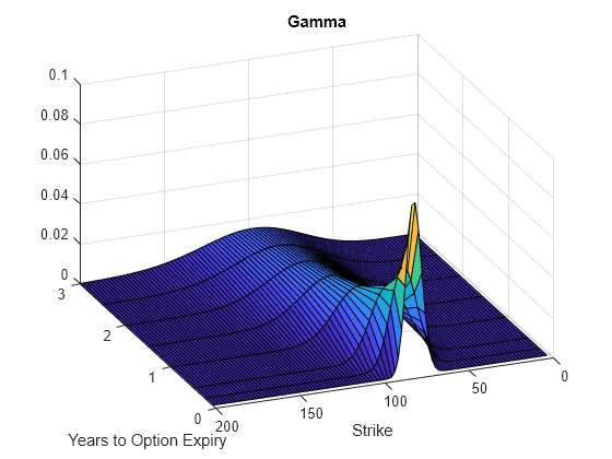
Plot Option Sensitivity Surfaces

Use the Strike input to specify the strikes. Increase the value for NumFFT to support a wider range of strikes. Also, the Maturity input can be a vector. Set ExpandOutput to "true" to output the surfaces as NStrikes-by-NMaturities matrices.

Settle = datetime(2017,6,29);
Maturity = datemnth(Settle, 12*[1/12 0.25 (0.5:0.5:3)]');
Times = yearfrac(Settle, Maturity);
Strike = (2:2:200)';

% Increase 'NumFFT' to support a wider range of strikes
NumFFT = 2^13;

[Delta, Gamma, Rho, Theta, Vega, VegaLT] = ...
    optSensByHestonFFT(Rate, AssetPrice, Settle, Maturity, OptSpec, Strike, ...
    V0, ThetaV, Kappa, SigmaV, RhoSV, 'DividendYield', DividendYield, 'NumFFT', NumFFT, ...
    'CharacteristicFcnStep', 0.065, 'LogStrikeStep', 0.001, 'ExpandOutput', true, ...
    'OutSpec', ["delta", "gamma", "rho", "theta", "vega", "vegalt"]);

[X,Y] = meshgrid(Times,Strike);

figure;
surf(X,Y,Delta);
title('Delta');
xlabel('Years to Option Expiry');
ylabel('Strike');
view(-112,34);
xlim([0 Times(end)]);

Figure contains an axes object. The axes object with title Delta, xlabel Years to Option Expiry, ylabel Strike contains an object of type surface.

figure;
surf(X,Y,Gamma)
title('Gamma')
xlabel('Years to Option Expiry')
ylabel('Strike')
view(-112,34);
xlim([0 Times(end)]);

Figure contains an axes object. The axes object with title Gamma, xlabel Years to Option Expiry, ylabel Strike contains an object of type surface.

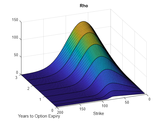
figure;
surf(X,Y,Rho)
title('Rho')
xlabel('Years to Option Expiry')
ylabel('Strike')
view(-112,34);
xlim([0 Times(end)]);

Figure contains an axes object. The axes object with title Rho, xlabel Years to Option Expiry, ylabel Strike contains an object of type surface.

figure;
surf(X,Y,Theta)
title('Theta')
xlabel('Years to Option Expiry')
ylabel('Strike')
view(-112,34);
xlim([0 Times(end)]);

Figure contains an axes object. The axes object with title Theta, xlabel Years to Option Expiry, ylabel Strike contains an object of type surface.

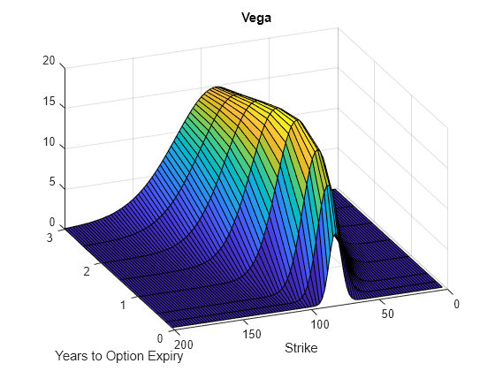
figure;
surf(X,Y,Vega)
title('Vega')
xlabel('Years to Option Expiry')
ylabel('Strike')
view(-112,34);
xlim([0 Times(end)]);

Figure contains an axes object. The axes object with title Vega, xlabel Years to Option Expiry, ylabel Strike contains an object of type surface.

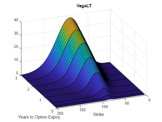
figure;
surf(X,Y,VegaLT)
title('VegaLT')
xlabel('Years to Option Expiry')
ylabel('Strike')
view(-112,34);
xlim([0 Times(end)]);

Figure contains an axes object. The axes object with title VegaLT, xlabel Years to Option Expiry, ylabel Strike contains an object of type surface.

Input Arguments

collapse all

Continuously compounded risk-free interest rate, specified as a scalar decimal value.

Data Types: double

Current underlying asset price, specified as numeric value using a scalar or a NINST-by-1 or NColumns-by-1 vector.

For more information on the proper dimensions for AssetPrice, see the name-value pair argument ExpandOutput.

Data Types: double

Option settlement date, specified as a NINST-by-1 or NColumns-by-1 vector using a datetime array, string array, or date character vectors. The Settle date must be before the Maturity date.

To support existing code, optSensByHestonFFT also accepts serial date numbers as inputs, but they are not recommended.

For more information on the proper dimensions for Settle, see the name-value pair argument ExpandOutput.

Option maturity date, specified as a NINST-by-1 or NColumns-by-1 vector using a datetime array, string array, or date character vectors.

To support existing code, optSensByHestonFFT also accepts serial date numbers as inputs, but they are not recommended.

For more information on the proper dimensions for Maturity, see the name-value pair argument ExpandOutput.

Definition of the option, specified as a NINST-by-1 or NColumns-by-1 vector using a cell array of character vectors or string arrays with values 'call' or 'put'.

For more information on the proper dimensions for OptSpec, see the name-value pair argument ExpandOutput.

Data Types: cell | string

Option strike price value, specified as a NINST-by-1, NRows-by-1, NRows-by-NColumns vector of strike prices.

If this input is an empty array ([]), option prices are computed on the entire FFT (or FRFT) strike grid, which is determined as exp(log-strike grid). Each column of the log-strike grid has 'NumFFT' points with 'LogStrikeStep' spacing that are roughly centered around each element of log(AssetPrice).

For more information on the proper dimensions for Strike, see the name-value pair argument ExpandOutput.

Data Types: double

Initial variance of the underling asset, specified as a scalar numeric value.

Data Types: double

Long-term variance of the underling asset, specified as a scalar numeric value.

Data Types: double

Mean revision speed for the underling asset, specified as a scalar numeric value.

Data Types: double

Volatility of the variance of the underling asset, specified as a scalar numeric value.

Data Types: double

Correlation between the Wiener processes for the underlying asset and its variance, specified as a scalar numeric value.

Data Types: double

Name-Value Arguments

Specify optional pairs of arguments as Name1=Value1,...,NameN=ValueN, where Name is the argument name and Value is the corresponding value. Name-value arguments must appear after other arguments, but the order of the pairs does not matter.

Before R2021a, use commas to separate each name and value, and enclose Name in quotes.

Example: [PriceSens,StrikeOut] = optSensByHestonFFT(Rate, AssetPrice,Settle,Maturity,OptSpec,Strike,V0,ThetaV,Kappa,SigmaV,RhoSV,'Basis',7,'OptSpec',"vega")

Day-count of the instrument, specified as the comma-separated pair consisting of 'Basis' and a scalar using a supported value:

  • 0 = actual/actual

  • 1 = 30/360 (SIA)

  • 2 = actual/360

  • 3 = actual/365

  • 4 = 30/360 (PSA)

  • 5 = 30/360 (ISDA)

  • 6 = 30/360 (European)

  • 7 = actual/365 (Japanese)

  • 8 = actual/actual (ICMA)

  • 9 = actual/360 (ICMA)

  • 10 = actual/365 (ICMA)

  • 11 = 30/360E (ICMA)

  • 12 = actual/365 (ISDA)

  • 13 = BUS/252

For more information, see Basis.

Data Types: double

Continuously compounded underlying asset yield, specified as the comma-separated pair consisting of 'DividendYield' and a scalar numeric value.

Data Types: double

Volatility risk premium, specified as the comma-separated pair consisting of 'VolRiskPremium' and a scalar numeric value.

Data Types: double

Flag indicating Little Heston Trap formulation by Albrecher et al, specified as the comma-separated pair consisting of 'LittleTrap' and a logical:

  • true — Use the Albrecher et al formulation.

  • false — Use the original Heston formation.

Data Types: logical

Define outputs, specified as the comma-separated pair consisting of 'OutSpec' and a NOUT- by-1 or a 1-by-NOUT string array or cell array of character vectors with supported values.

Note

"vega" is the sensitivity with respect the initial volatility sqrt(V0). In contrast, "vegalt" is the sensitivity with respect to the long-term volatility sqrt(ThetaV).

Example: OutSpec = ["price","delta","gamma","vega","rho","theta","vegalt"]

Data Types: string | cell

Number of grid points in the characteristic function variable and in each column of the log-strike grid, specified as the comma-separated pair consisting of 'NumFFT' and a scalar numeric value.

Data Types: double

Characteristic function variable grid spacing, specified as the comma-separated pair consisting of 'CharacteristicFcnStep' and a scalar numeric value.

Data Types: double

Log-strike grid spacing, specified as the comma-separated pair consisting of 'LogStrikeStep' and a scalar numeric value.

Note

If (LogStrikeStep*CharacteristicFcnStep) is 2*pi/NumFFT, FFT is used. Otherwise, FRFT is used.

Data Types: double

Damping factor for Carr-Madan formulation, specified as the comma-separated pair consisting of 'DampingFactor' and a scalar numeric value.

Data Types: double

Type of quadrature, specified as the comma-separated pair consisting of 'Quadrature' and a single character vector or string array with a value of simpson or trapezoidal.

Data Types: char | string

Flag to expand the outputs, specified as the comma-separated pair consisting of 'ExpandOutput' and a logical:

  • true — If true, the outputs are NRows-by- NColumns matrices. NRows is the number of strikes for each column and it is determined by the Strike input. For example, Strike can be a NRows-by-1 vector, or a NRows-by-NColumns matrix. If Strike is empty, NRows is equal to NumFFT. NColumns is determined by the sizes of AssetPrice, Settle, Maturity, and OptSpec, which must all be either scalar or NColumns-by-1 vectors.

  • false — If false, the outputs are NINST-by-1 vectors. Also, the inputs Strike, AssetPrice, Settle, Maturity, and OptSpec must all be either scalar or NINST-by-1 vectors.

Data Types: logical

Output Arguments

collapse all

Option prices or sensitivities, returned as a NINST-by-1, or NRows-by-NColumns, depending on ExpandOutput. The name-value pair argument OutSpec determines the types and order of the outputs.

Strikes corresponding to Price, returned as a NINST-by-1, or NRows-by-NColumns, depending on ExpandOutput.

More About

collapse all

Vanilla Option

A vanilla option is a category of options that includes only the most standard components.

A vanilla option has an expiration date and straightforward strike price. American-style options and European-style options are both categorized as vanilla options.

The payoff for a vanilla option is as follows:

  • For a call: max(StK,0)

  • For a put: max(KSt,0)

where:

St is the price of the underlying asset at time t.

K is the strike price.

For more information, see Vanilla Option.

Heston Stochastic Volatility Model

The Heston model is an extension of the Black-Scholes model, where the volatility (square root of variance) is no longer assumed to be constant, and the variance now follows a stochastic (CIR) process. This process allows modeling the implied volatility smiles observed in the market.

The stochastic differential equation is:

dSt=(rq)Stdt+vtStdWtdvt=κ(θvt)dt+σvvtdWtvE[dWtdWtv]=pdt

where

r is the continuous risk-free rate.

q is the continuous dividend yield.

St is the asset price at time t.

vt is the asset price variance at time t

v0 is the initial variance of the asset price at t = 0 for (v0 > 0).

θ is the long-term variance level for (θ > 0).

κ is the mean reversion speed for the variance for (κ > 0).

σv is the volatility of the variance for (σv > 0).

p is the correlation between the Wiener processes Wt and Wvt for (-1 ≤ p ≤ 1).

The characteristic function fHestonj(ϕ) for j = 1 (asset price measure) and j = 2 (risk-neutral measure) is:

fHestonj(ϕ)=exp(Cj+Djv0+iϕlnSt)Cj=(rq)iϕτ+κθσv2[(bjpσviϕ+dj)τ2ln(1gjedjτ1gj)]Dj=bjpσviϕ+djσv2(1edjτ1gjedjτ)gj=bjpσviϕ+djbjpσviϕdjdj=(bjpσviϕ)2σv2(2ujiϕϕ2)where for j=1,2:u1=12,u2=12,b1=κ+λVolRiskpσv,b2=κ+λVolRisk

where

ϕ is the characteristic function variable.

ƛVolRisk is the volatility risk premium.

τ is the time to maturity (τ = T - t).

i is the unit imaginary number (i2 = -1).

The definitions for Cj and Dj under “The Little Heston Trap” by Albrecher et al. (2007) are:

Cj=(rq)iϕτ+κθσv2[(bjpσviϕdj)τ2ln(1εjedjτ1εj)]Dj=bjpσviϕdjσv2(1edjτ1εjedjτ)εj=bjpσviϕdjbjpσviϕ+dj

Carr-Madan Formulation

The Carr and Madan (1999) formulation is a popular modified implementation of Heston (1993) framework.

Rather than computing the probabilities P1 and P2 as intermediate steps, Carr and Madan developed an alternative expression so that taking its inverse Fourier transform gives the option price itself directly.

Call(k)=eαkπ0Re[eiukψ(u)]duψ(u)=erτf2(ϕ=(u(α+1)i))α2+αu2+iu(2α+1)Put(K)=Call(K)+KerτSteqτ

where

r is the continuous risk-free rate.

q is the continuous dividend yield.

St is the asset price at time t.

τ is time to maturity (τ = T-t).

Call(K) is the call price at strike K.

Put(K) is the put price at strike K.

i is a unit imaginary number (i2= -1).

ϕ is the characteristic function variable.

α is the damping factor.

u is the characteristic function variable for integration, where ϕ = (u - (α+1)i).

f2(ϕ) is the characteristic function for P2.

P2 is the probability of St > K under the risk-neutral measure for the model.

To apply FFT or FRFT to this formulation, the characteristic function variable for integration, u, is discretized into NumFFT(N) points with the step size CharacteristicFcnStepu), and the log-strike k is discretized into N points with the step size LogStrikeStepk).

The discretized characteristic function variable for integration, uj(for j = 1,2,3,…,N), has a minimum value of 0 and a maximum value of (N-1) (Δu), and it approximates the continuous integration range from 0 to infinity.

The discretized log-strike grid, kn(for n = 1, 2, 3, N) is approximately centered around ln(St), with a minimum value of

ln(St)N2Δk

and a maximum value of

ln(St)+(N21)Δk

Where the minimum allowable strike is

Stexp(N2Δk)

and the maximum allowable strike is

Stexp[(N21)Δk]

As a result of the discretization, the expression for the call option becomes

Call(kn)=Δueαknπj=1NRe[eiΔkΔu(j1)(n1)eiuj[NΔk2ln(St)]ψ(uj)]wj

where

Δu is the step size of discretized characteristic function variable for integration.

Δk is the step size of discretized log-strike.

N is the number of FFT or FRFT points.

wj is the weights for quadrature used for approximating the integral.

FFT is used to evaluate the above expression if Δk and Δu are subject to the following constraint:

ΔkΔu=(2πN)

otherwise, the functions use the FRFT method described in Chourdakis (2005).

References

[1] Albrecher, H., Mayer, P., Schoutens, W., and Tistaert, J. "The Little Heston Trap." Working Paper, Linz and Graz University of Technology, K.U. Leuven, ING Financial Markets, 2006.

[2] Carr, P. and D.B. Madan. “Option Valuation using the Fast Fourier Transform.” Journal of Computational Finance. Vol 2. No. 4. 1999.

[3] Chourdakis, K. “Option Pricing Using Fractional FFT.” Journal of Computational Finance. 2005.

[4] Heston, S. L. “A Closed-Form Solution for Options with Stochastic Volatility with Applications to Bond and Currency Options.” The Review of Financial Studies. Vol 6. No. 2. 1993.

Version History

Introduced in R2018a

expand all