Track-Level Fusion of Radar and Lidar Data
This example shows you how to generate an object-level track list from measurements of a radar and a lidar sensor and further fuse them using a track-level fusion scheme. You process the radar measurements using an extended object tracker and the lidar measurements using a joint probabilistic data association (JPDA) tracker. You further fuse these tracks using a track-level fusion scheme. The schematic of the workflow is shown below.

See Fusion of Radar and Lidar Data Using ROS (ROS Toolbox) for an example of this algorithm using recorded data on a rosbag.
Setup Scenario for Synthetic Data Generation
The scenario used in this example is created using drivingScenario (Automated Driving Toolbox). The data from radar and lidar sensors is simulated using drivingRadarDataGenerator (Automated Driving Toolbox) and lidarPointCloudGenerator (Automated Driving Toolbox), respectively. The creation of the scenario and the sensor models is wrapped in the helper function helperCreateRadarLidarScenario. For more information on scenario and synthetic data generation, refer to Create Driving Scenario Programmatically (Automated Driving Toolbox).
% For reproducible results
rng(2021);

% Create scenario, ego vehicle and get radars and lidar sensor
[scenario, egoVehicle, radars, lidar] = helperCreateRadarLidarScenario;
The ego vehicle is mounted with four 2-D radar sensors. The front and rear radar sensors have a field of view of 45 degrees. The left and right radar sensors have a field of view of 150 degrees. Each radar has a resolution of 6 degrees in azimuth and 2.5 meters in range. The ego is also mounted with one 3-D lidar sensor with a field of view of 360 degrees in azimuth and 40 degrees in elevation. The lidar has a resolution of 0.2 degrees in azimuth and 1.25 degrees in elevation (32 elevation channels). Visualize the configuration of the sensors and the simulated sensor data in the animation below. Notice that the radars have higher resolution than objects and therefore return multiple measurements per object. Also notice that the lidar interacts with the low-poly mesh of the actor as well as the road surface to return multiple points from these objects.

Radar Tracking Algorithm
As mentioned, the radars have higher resolution than the objects and return multiple detections per object. Conventional trackers such as Global Nearest Neighbor (GNN) and Joint Probabilistic Data Association (JPDA) assume that the sensors return at most one detection per object per scan. Therefore, the detections from high-resolution sensors must be either clustered before processing it with conventional trackers or must be processed using extended object trackers. Extended object trackers do not require pre-clustering of detections and usually estimate both kinematic states (for example, position and velocity) and the extent of the objects. For a more detailed comparison between conventional trackers and extended object trackers, refer to the Extended Object Tracking of Highway Vehicles with Radar and Camera example.
In general, extended object trackers offer better estimation of objects as they handle clustering and data association simultaneously using temporal history of tracks. In this example, the radar detections are processed using a Gaussian mixture probability hypothesis density (GM-PHD) tracker (trackerPHD and gmphd) with a rectangular target model. For more details on configuring the tracker, refer to the "GM-PHD Rectangular Object Tracker" section of the Extended Object Tracking of Highway Vehicles with Radar and Camera example.
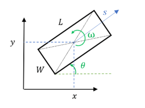
The algorithm for tracking objects using radar measurements is wrapped inside the helper class, helperRadarTrackingAlgorithm, implemented as a System object™. This class outputs an array of objectTrack objects and define their state according to the following convention:
![$[x\ y\ s\ {\theta}\ {\omega}\ L\ W]$](../../examples/shared_driving_fusion_lidar/win64/RadarAndLidarTrackFusionExample_eq08379674716755000917.png)
radarTrackingAlgorithm = helperRadarTrackingAlgorithm(radars);
Lidar Tracking Algorithm
Similar to radars, the lidar sensor also returns multiple measurements per object. Further, the sensor returns a large number of points from the road, which must be removed before used as inputs for an object-tracking algorithm. While lidar data from obstacles can be directly processed via extended object tracking algorithm, conventional tracking algorithms are still more prevalent for tracking using lidar data. The first reason for this trend is mainly observed due to higher computational complexity of extended object trackers for large data sets. The second reason is the investments into advanced Deep learning-based detectors such as PointPillars [1], VoxelNet [2] and PIXOR [3], which can segment a point cloud and return bounding box detections for the vehicles. These detectors can help in overcoming the performance degradation of conventional trackers due to improper clustering.
In this example, the lidar data is processed using a conventional joint probabilistic data association (JPDA) tracker, configured with an interacting multiple model (IMM) filter. The pre-processing of lidar data to remove point cloud is performed by using a RANSAC-based plane-fitting algorithm and bounding boxes are formed by performing a Euclidian-based distance clustering algorithm. For more information about the algorithm, refer to the Track Vehicles Using Lidar: From Point Cloud to Track List example. Compared the linked example, the tracking is performed in the scenario frame and the tracker is tuned differently to track objects of different sizes. Further the states of the variables are defined differently to constrain the motion of the tracks in the direction of its estimated heading angle.
The algorithm for tracking objects using lidar data is wrapped inside the helper class, helperLidarTrackingAlgorithm implemented as System object. This class outputs an array of objectTrack objects and defines their state according to the following convention:
![$[x\ y\ s\ {\theta}\ {\omega}\ z\ {\dot{z}}\ L\ W\ H]$](../../examples/shared_driving_fusion_lidar/win64/RadarAndLidarTrackFusionExample_eq16648117378020166922.png)
The states common to the radar algorithm are defined similarly. Also, as a 3-D sensor, the lidar tracker outputs three additional states,  ,
,  and
and  , which refer to z-coordinate (m), z-velocity (m/s), and height (m) of the tracked object respectively.
lidarTrackingAlgorithm = helperLidarTrackingAlgorithm(lidar);
Set Up Fuser, Metrics, and Visualization
Fuser
Next, you will set up a fusion algorithm for fusing the list of tracks from radar and lidar trackers. Similar to other tracking algorithms, the first step towards setting up a track-level fusion algorithm is defining the choice of state vector (or state-space) for the fused or central tracks. In this case, the state-space for fused tracks is chosen to be same as the lidar. After choosing a central track state-space, you define the transformation of the central track state to the local track state. In this case, the local track state-space refers to states of radar and lidar tracks. To do this, you use a fuserSourceConfiguration object.
Define the configuration of the radar source. The helperRadarTrackingAlgorithm outputs tracks with SourceIndex set to 1. The SourceIndex is provided as a property on each tracker to uniquely identify it and allows a fusion algorithm to distinguish tracks from different sources. Therefore, you set the SourceIndex property of the radar configuration as same as those of the radar tracks. You set IsInitializingCentralTracks to true to let that unassigned radar tracks initiate new central tracks. Next, you define the transformation of a track in central state-space to the radar state-space and vice-versa. The helper functions central2radar and radar2central perform the two transformations and are included at the end of this example.
radarConfig = fuserSourceConfiguration('SourceIndex',1,...
    'IsInitializingCentralTracks',true,...
    'CentralToLocalTransformFcn',@central2radar,...
    'LocalToCentralTransformFcn',@radar2central);
Define the configuration of the lidar source. Since the state-space of a lidar track is same as central track, you do not define any transformations.
lidarConfig = fuserSourceConfiguration('SourceIndex',2,...
    'IsInitializingCentralTracks',true);
The next step is to define the state-fusion algorithm. The state-fusion algorithm takes multiple states and state covariances in the central state-space as input and returns a fused estimate of the state and the covariances. In this example, you use a covariance intersection algorithm provided by the helper function, helperRadarLidarFusionFcn. A generic covariance intersection algorithm for two Gaussian estimates with mean  and covariance
  can be defined according to the following equations:


where  and
and  are the fused state and covariance and
  and
and  are mixing coefficients from each estimate. Typically, these mixing coefficients are estimated by minimizing the determinant or the trace of the fused covariance. In this example, the mixing weights are estimated by minimizing the determinant of positional covariance of each estimate. Furthermore, as the radar does not estimate 3-D states, 3-D states are only fused with lidars. For more details, refer to the
 helperRadarLidarFusionFcn function shown at the end of this script.
Next, you assemble all the information using a trackFuser object.
% The state-space of central tracks is same as the tracks from the lidar,
% therefore you use the same state transition function. The function is
% defined inside the helperLidarTrackingAlgorithm class.
f = lidarTrackingAlgorithm.StateTransitionFcn;

% Create a trackFuser object
fuser = trackFuser('SourceConfigurations',{radarConfig;lidarConfig},...
    'StateTransitionFcn',f,...
    'ProcessNoise',diag([1 3 1]),...
    'HasAdditiveProcessNoise',false,...
    'AssignmentThreshold',[250 inf],...
    'ConfirmationThreshold',[3 5],...
    'DeletionThreshold',[5 5],...
    'StateFusion','Custom',...
    'CustomStateFusionFcn',@helperRadarLidarFusionFcn);
Metrics
In this example, you assess the performance of each algorithm using the Generalized Optimal SubPattern Assignment Metric (GOSPA) metric. You set up three separate metrics using trackGOSPAMetric for each of the trackers. The GOSPA metric aims to evaluate the performance of a tracking system by providing a scalar cost. A lower value of the metric indicates better performance of the tracking algorithm.
To use the GOSPA metric with custom motion models like the one used in this example, you set the Distance property to 'custom' and define a distance function between a track and its associated ground truth. These distance functions, shown at the end of this example are helperRadarDistance, and helperLidarDistance.
% Radar GOSPA
gospaRadar = trackGOSPAMetric('Distance','custom',...
    'DistanceFcn',@helperRadarDistance,...
    'CutoffDistance',25);

% Lidar GOSPA
gospaLidar = trackGOSPAMetric('Distance','custom',...
    'DistanceFcn',@helperLidarDistance,...
    'CutoffDistance',25);

% Central/Fused GOSPA
gospaCentral = trackGOSPAMetric('Distance','custom',...
    'DistanceFcn',@helperLidarDistance,...% State-space is same as lidar
    'CutoffDistance',25);
Visualization
The visualization for this example is implemented using a helper class helperLidarRadarTrackFusionDisplay. The display is divided into 4 panels. The display plots the measurements and tracks from each sensor as well as the fused track estimates. The legend for the display is shown below. Furthermore, the tracks are annotated by their unique identity (TrackID) as well as a prefix. The prefixes "R", "L" and "F" stand for radar, lidar, and fused estimate, respectively.
% Create a display.
% FollowActorID controls the actor shown in the close-up
% display
display = helperLidarRadarTrackFusionDisplay('FollowActorID',3);

% Show persistent legend
showLegend(display,scenario);

Run Scenario and Trackers
Next, you advance the scenario, generate synthetic data from all sensors and process it to generate tracks from each of the systems. You also compute the metric for each tracker using the ground truth available from the scenario.
% Initialize GOSPA metric and its components for all tracking algorithms.
gospa = zeros(3,0);
missTarget = zeros(3,0);
falseTracks = zeros(3,0);

% Initialize fusedTracks
fusedTracks = objectTrack.empty(0,1);

% A counter for time steps elapsed for storing gospa metrics.
idx = 1;

% Ground truth for metrics. This variable updates every time-step
% automatically being a handle to the actors.
groundTruth = scenario.Actors(2:end);

while advance(scenario)
    % Current time
    time = scenario.SimulationTime;

    % Collect radar and lidar measurements and ego pose to track in
    % scenario frame. See helperCollectSensorData below.
    [radarDetections, ptCloud, egoPose] = helperCollectSensorData(egoVehicle, radars, lidar, time);

    % Generate radar tracks
    radarTracks = radarTrackingAlgorithm(egoPose, radarDetections, time);

    % Generate lidar tracks and analysis information like bounding box
    % detections and point cloud segmentation information
    [lidarTracks, lidarDetections, segmentationInfo] = ...
        lidarTrackingAlgorithm(egoPose, ptCloud, time);

    % Concatenate radar and lidar tracks
    localTracks = [radarTracks;lidarTracks];

    % Update the fuser. First call must contain one local track
    if ~(isempty(localTracks) && ~isLocked(fuser))
        fusedTracks = fuser(localTracks,time);
    end

    % Capture GOSPA and its components for all trackers
    [gospa(1,idx),~,~,~,missTarget(1,idx),falseTracks(1,idx)] = gospaRadar(radarTracks, groundTruth);
    [gospa(2,idx),~,~,~,missTarget(2,idx),falseTracks(2,idx)] = gospaLidar(lidarTracks, groundTruth);
    [gospa(3,idx),~,~,~,missTarget(3,idx),falseTracks(3,idx)] = gospaCentral(fusedTracks, groundTruth);

    % Update the display
    display(scenario, radars, radarDetections, radarTracks, ...
        lidar, ptCloud, lidarDetections, segmentationInfo, lidarTracks,...
        fusedTracks);

    % Update the index for storing GOSPA metrics
    idx = idx + 1;
end

% Update example animations
updateExampleAnimations(display);
Evaluate Performance
Evaluate the performance of each tracker using visualization as well as quantitative metrics. Analyze different events in the scenario and understand how the track-level fusion scheme helps achieve a better estimation of the vehicle state.
Track Maintenance
The animation below shows the entire run every three time-steps. Note that each of the three tracking systems - radar, lidar, and the track-level fusion - were able to track all four vehicles in the scenario and no false tracks were confirmed.

You can also quantitatively measure this aspect of the performance using "missed target" and "false track" components of the GOSPA metric. Notice in the figures below that missed target component starts from a higher value due to establishment delay and goes down to zero in about 5-10 steps for each tracking system. Also, notice that the false track component is zero for all systems, which indicates that no false tracks were confirmed.
% Plot missed target component
figure; plot(missTarget','LineWidth',2); legend('Radar','Lidar','Fused');
title("Missed Target Metric"); xlabel('Time step'); ylabel('Metric'); grid on;

% Plot false track component
figure; plot(falseTracks','LineWidth',2); legend('Radar','Lidar','Fused');
title("False Track Metric"); xlabel('Time step'); ylabel('Metric'); grid on;


Track-level Accuracy
The track-level or localization accuracy of each tracker can also be quantitatively assessed by the GOSPA metric at each time step. A lower value indicates better tracking accuracy. As there were no missed targets or false tracks, the metric captures the localization errors resulting from state estimation of each vehicle.
Note that the GOSPA metric for fused estimates is lower than the metric for individual sensor, which indicates that track accuracy increased after fusion of track estimates from each sensor.
% Plot GOSPA
figure; plot(gospa','LineWidth',2); legend('Radar','Lidar','Fused');
title("GOSPA Metric"); xlabel('Time step'); ylabel('Metric'); grid on;

Closely-spaced targets
As mentioned earlier, this example uses a Euclidian-distance based clustering and bounding box fitting to feed the lidar data to a conventional tracking algorithm. Clustering algorithms typically suffer when objects are closely-spaced. With the detector configuration used in this example, when the passing vehicle approaches the vehicle in front of the ego vehicle, the detector clusters the point cloud from each vehicle into a bigger bounding box. You can notice in the animation below that the track drifted away from the vehicle center. Because the track was reported with higher certainty in its estimate for a few steps, the fused estimated was also affected initially. However, as the uncertainty increases, its association with the fused estimate becomes weaker. This is because the covariance intersection algorithm chooses a mixing weight for each assigned track based on the certainty of each estimate.

This effect is also captured in the GOSPA metric. You can notice in the GOSPA metric plot above that the lidar metric shows a peak around the 65th time step.
The radar tracks are not affected during this event because of two main reasons. Firstly, the radar sensor outputs range-rate information in each detection, which is different beyond noise-levels for the passing car as compared to the slower moving car. This results in an increased statistical distance between detections from individual cars. Secondly, extended object trackers evaluate multiple possible clustering hypothesis against predicted tracks, which results in rejection of improper clusters and acceptance of proper clusters. Note that for extended object trackers to properly choose the best clusters, the filter for the track must be robust to a degree that can capture the difference between two clusters. For example, a track with high process noise and highly uncertain dimensions may not be able to properly claim a cluster because of its premature age and higher flexibility to account for uncertain events.
Targets at long range
As targets recede away from the radar sensors, the accuracy of the measurements degrade because of reduced signal-to-noise ratio at the detector and the limited resolution of the sensor. This results in high uncertainty in the measurements, which in turn reduces the track accuracy. Notice in the close-up display below that the track estimate from the radar is further away from the ground truth for the radar sensor and is reported with a higher uncertainty. However, the lidar sensor reports enough measurements in the point cloud to generate a "shrunk" bounding box. The shrinkage effect modeled in the measurement model for lidar tracking algorithm allows the tracker to maintain a track with correct dimensions. In such situations, the lidar mixing weight is higher than the radar and allows the fused estimate to be more accurate than the radar estimate.

Summary
In this example, you learned how to set up a track-level fusion algorithm for fusing tracks from radar and lidar sensors. You also learned how to evaluate a tracking algorithm using the Generalized Optimal Subpattern Metric and its associated components.
Utility Functions
collectSensorData
A function to generate radar and lidar measurements at the current time-step.
function [radarDetections, ptCloud, egoPose] = helperCollectSensorData(egoVehicle, radars, lidar, time)

% Current poses of targets with respect to ego vehicle
tgtPoses = targetPoses(egoVehicle);

radarDetections = cell(0,1);
for i = 1:numel(radars)
    thisRadarDetections = step(radars{i},tgtPoses,time);
    radarDetections = [radarDetections;thisRadarDetections]; %#ok<AGROW>
end

% Generate point cloud from lidar
rdMesh = roadMesh(egoVehicle);
ptCloud = step(lidar, tgtPoses, rdMesh, time);

% Compute pose of ego vehicle to track in scenario frame. Typically
% obtained using an INS system. If unavailable, this can be set to
% "origin" to track in ego vehicle's frame.
egoPose = pose(egoVehicle);

end
radar2cental
A function to transform a track in the radar state-space to a track in the central state-space.
function centralTrack = radar2central(radarTrack)

% Initialize a track of the correct state size
centralTrack = objectTrack('State',zeros(10,1),...
    'StateCovariance',eye(10));

% Sync properties of radarTrack except State and StateCovariance with
% radarTrack See syncTrack defined below.
centralTrack = syncTrack(centralTrack,radarTrack);

xRadar = radarTrack.State;
PRadar = radarTrack.StateCovariance;

H = zeros(10,7); % Radar to central linear transformation matrix
H(1,1) = 1;
H(2,2) = 1;
H(3,3) = 1;
H(4,4) = 1;
H(5,5) = 1;
H(8,6) = 1;
H(9,7) = 1;

xCentral = H*xRadar;  % Linear state transformation
PCentral = H*PRadar*H'; % Linear covariance transformation

PCentral([6 7 10],[6 7 10]) = eye(3); % Unobserved states

% Set state and covariance of central track
centralTrack.State = xCentral;
centralTrack.StateCovariance = PCentral;

end
central2radar
A function to transform a track in the central state-space to a track in the radar state-space.
function radarTrack = central2radar(centralTrack)

% Initialize a track of the correct state size
radarTrack = objectTrack('State',zeros(7,1),...
    'StateCovariance',eye(7));

% Sync properties of centralTrack except State and StateCovariance with
% radarTrack See syncTrack defined below.
radarTrack = syncTrack(radarTrack,centralTrack);

xCentral = centralTrack.State;
PCentral = centralTrack.StateCovariance;

H = zeros(7,10); % Central to radar linear transformation matrix
H(1,1) = 1;
H(2,2) = 1;
H(3,3) = 1;
H(4,4) = 1;
H(5,5) = 1;
H(6,8) = 1;
H(7,9) = 1;

xRadar = H*xCentral;  % Linear state transformation
PRadar = H*PCentral*H'; % Linear covariance transformation

% Set state and covariance of radar track
radarTrack.State = xRadar;
radarTrack.StateCovariance = PRadar;
end
syncTrack
A function to syncs properties of one track with another except the State and StateCovariance properties.
function tr1 = syncTrack(tr1,tr2)
props = properties(tr1);
notState = ~strcmpi(props,'State');
notCov = ~strcmpi(props,'StateCovariance');

props = props(notState & notCov);
for i = 1:numel(props)
    tr1.(props{i}) = tr2.(props{i});
end
end
pose
A function to return pose of the ego vehicle as a structure.
function egoPose = pose(egoVehicle)
egoPose.Position = egoVehicle.Position;
egoPose.Velocity = egoVehicle.Velocity;
egoPose.Yaw = egoVehicle.Yaw;
egoPose.Pitch = egoVehicle.Pitch;
egoPose.Roll = egoVehicle.Roll;
end
helperLidarDistance
Function to calculate a normalized distance between the estimate of a track in radar state-space and the assigned ground truth.
function dist = helperLidarDistance(track, truth)

% Calculate the actual values of the states estimated by the tracker

% Center is different than origin and the trackers estimate the center
rOriginToCenter = -truth.OriginOffset(:) + [0;0;truth.Height/2];
rot = quaternion([truth.Yaw truth.Pitch truth.Roll],'eulerd','ZYX','frame');
actPos = truth.Position(:) + rotatepoint(rot,rOriginToCenter')';

% Actual speed and z-rate
actVel = [norm(truth.Velocity(1:2));truth.Velocity(3)];

% Actual yaw
actYaw = truth.Yaw;

% Actual dimensions.
actDim = [truth.Length;truth.Width;truth.Height];

% Actual yaw rate
actYawRate = truth.AngularVelocity(3);

% Calculate error in each estimate weighted by the "requirements" of the
% system. The distance specified using Mahalanobis distance in each aspect
% of the estimate, where covariance is defined by the "requirements". This
% helps to avoid skewed distances when tracks under/over report their
% uncertainty because of inaccuracies in state/measurement models.

% Positional error.
estPos = track.State([1 2 6]);
reqPosCov = 0.1*eye(3);
e = estPos - actPos;
d1 = sqrt(e'/reqPosCov*e);

% Velocity error
estVel = track.State([3 7]);
reqVelCov = 5*eye(2);
e = estVel - actVel;
d2 = sqrt(e'/reqVelCov*e);

% Yaw error
estYaw = track.State(4);
reqYawCov = 5;
e = estYaw - actYaw;
d3 = sqrt(e'/reqYawCov*e);

% Yaw-rate error
estYawRate = track.State(5);
reqYawRateCov = 1;
e = estYawRate - actYawRate;
d4 = sqrt(e'/reqYawRateCov*e);

% Dimension error
estDim = track.State([8 9 10]);
reqDimCov = eye(3);
e = estDim - actDim;
d5 = sqrt(e'/reqDimCov*e);

% Total distance
dist = d1 + d2 + d3 + d4 + d5;

end
helperRadarDistance
Function to calculate a normalized distance between the estimate of a track in radar state-space and the assigned ground truth.
function dist = helperRadarDistance(track, truth)

% Calculate the actual values of the states estimated by the tracker

% Center is different than origin and the trackers estimate the center
rOriginToCenter = -truth.OriginOffset(:) + [0;0;truth.Height/2];
rot = quaternion([truth.Yaw truth.Pitch truth.Roll],'eulerd','ZYX','frame');
actPos = truth.Position(:) + rotatepoint(rot,rOriginToCenter')';
actPos = actPos(1:2); % Only 2-D

% Actual speed
actVel = norm(truth.Velocity(1:2));

% Actual yaw
actYaw = truth.Yaw;

% Actual dimensions. Only 2-D for radar
actDim = [truth.Length;truth.Width];

% Actual yaw rate
actYawRate = truth.AngularVelocity(3);

% Calculate error in each estimate weighted by the "requirements" of the
% system. The distance specified using Mahalanobis distance in each aspect
% of the estimate, where covariance is defined by the "requirements". This
% helps to avoid skewed distances when tracks under/over report their
% uncertainty because of inaccuracies in state/measurement models.

% Positional error
estPos = track.State([1 2]);
reqPosCov = 0.1*eye(2);
e = estPos - actPos;
d1 = sqrt(e'/reqPosCov*e);

% Speed error
estVel = track.State(3);
reqVelCov = 5;
e = estVel - actVel;
d2 = sqrt(e'/reqVelCov*e);

% Yaw error
estYaw = track.State(4);
reqYawCov = 5;
e = estYaw - actYaw;
d3 = sqrt(e'/reqYawCov*e);

% Yaw-rate error
estYawRate = track.State(5);
reqYawRateCov = 1;
e = estYawRate - actYawRate;
d4 = sqrt(e'/reqYawRateCov*e);

% Dimension error
estDim = track.State([6 7]);
reqDimCov = eye(2);
e = estDim - actDim;
d5 = sqrt(e'/reqDimCov*e);

% Total distance
dist = d1 + d2 + d3 + d4 + d5;

% A constant penality for not measuring 3-D state
dist = dist + 3;

end
helperRadarLidarFusionFcn
Function to fuse states and state covariances in central track state-space
function [x,P] = helperRadarLidarFusionFcn(xAll,PAll)
n = size(xAll,2);
dets = zeros(n,1);

% Initialize x and P
x = xAll(:,1);
P = PAll(:,:,1);

onlyLidarStates = false(10,1);
onlyLidarStates([6 7 10]) = true;

% Only fuse this information with lidar
xOnlyLidar = xAll(onlyLidarStates,:);
POnlyLidar = PAll(onlyLidarStates,onlyLidarStates,:);

% States and covariances for intersection with radar and lidar both
xToFuse = xAll(~onlyLidarStates,:);
PToFuse = PAll(~onlyLidarStates,~onlyLidarStates,:);

% Sorted order of determinants. This helps to sequentially build the
% covariance with comparable determinations. For example, two large
% covariances may intersect to a smaller covariance, which is comparable to
% the third smallest covariance.
for i = 1:n
    dets(i) = det(PToFuse(1:2,1:2,i));
end
[~,idx] = sort(dets,'descend');
xToFuse = xToFuse(:,idx);
PToFuse = PToFuse(:,:,idx);

% Initialize fused estimate
thisX = xToFuse(:,1);
thisP = PToFuse(:,:,1);

% Sequential fusion
for i = 2:n
    [thisX,thisP] = fusecovintUsingPos(thisX, thisP, xToFuse(:,i), PToFuse(:,:,i));
end

% Assign fused states from all sources
x(~onlyLidarStates) = thisX;
P(~onlyLidarStates,~onlyLidarStates,:) = thisP;

% Fuse some states only with lidar source
valid = any(abs(xOnlyLidar) > 1e-6,1);
xMerge = xOnlyLidar(:,valid);
PMerge = POnlyLidar(:,:,valid);

if sum(valid) > 1
    [xL,PL] = fusecovint(xMerge,PMerge);
elseif sum(valid) == 1
    xL = xMerge;
    PL = PMerge;
else
    xL = zeros(3,1);
    PL = eye(3);
end

x(onlyLidarStates) = xL;
P(onlyLidarStates,onlyLidarStates) = PL;

end

function [x,P] = fusecovintUsingPos(x1,P1,x2,P2)
% Covariance intersection in general is employed by the following
% equations:
% P^-1 = w1*P1^-1 + w2*P2^-1
% x = P*(w1*P1^-1*x1 + w2*P2^-1*x2);
% where w1 + w2 = 1
% Usually a scalar representative of the covariance matrix like "det" or
% "trace" of P is minimized to compute w. This is offered by the function
% "fusecovint". However. in this case, the w are chosen by minimizing the
% determinants of "positional" covariances only.
n = size(x1,1);
idx = [1 2];
detP1pos = det(P1(idx,idx));
detP2pos = det(P2(idx,idx));
w1 = detP2pos/(detP1pos + detP2pos);
w2 = detP1pos/(detP1pos + detP2pos);
I = eye(n);

P1inv = I/P1;
P2inv = I/P2;

Pinv = w1*P1inv + w2*P2inv;
P = I/Pinv;

x = P*(w1*P1inv*x1 + w2*P2inv*x2);

end
References
[1] Lang, Alex H., et al. "PointPillars: Fast encoders for object detection from point clouds." Proceedings of the IEEE Conference on Computer Vision and Pattern Recognition. 2019.
[2] Zhou, Yin, and Oncel Tuzel. "Voxelnet: End-to-end learning for point cloud based 3d object detection." Proceedings of the IEEE Conference on Computer Vision and Pattern Recognition. 2018.
[3] Yang, Bin, Wenjie Luo, and Raquel Urtasun. "Pixor: Real-time 3d object detection from point clouds." Proceedings of the IEEE conference on Computer Vision and Pattern Recognition. 2018.