Centrifugal Pump (IL)

Centrifugal pump in isothermal liquid network

• 

Libraries:
Simscape / Fluids / Isothermal Liquid / Pumps & Motors

Description

The Centrifugal Pump (IL) block represents a centrifugal pump that transfers energy from the shaft to a fluid in an isothermal liquid network. The pressure differential and mechanical torque are functions of the pump head and brake power, which depend on pump capacity. You can parameterize the pump analytically or by linear interpolation of tabulated data. The pump affinity laws define the core physics of the block, which scale the pump performance to the ratio of the current to the reference values of the pump angular velocity and impeller diameter.

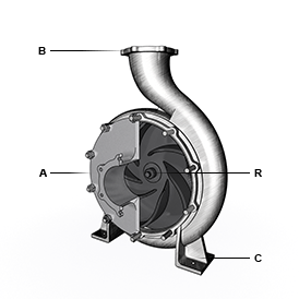
By default, the flow and pressure gain are from port A to port B. Port C represents the pump casing, and port R represents the pump shaft. You can specify the normal operating shaft direction in the Mechanical orientation parameter. If the shaft begins to spin in the opposite direction, the pressure difference across the block drops to zero.

Port Configuration

The figure shows the location of the block ports on a typical centrifugal pump.

Analytical Parameterization: Capacity, Head, and Brake Power

When you set, Pump parameterization to Capacity, head, and brake power at reference shaft speed, the block calculates the pressure gain over the pump as a function of the pump affinity laws and the reference pressure differential:

$$p_B-p_A=\Delta H_{ref}\rho g{\left(\frac{\omega }{{\omega }_{ref}}\right)}^2{\left(\frac{D}{D_{ref}}\right)}^2,$$

where:

• g is the gravitational acceleration.

• ΔH_ref is the reference pump head, which the block derives from a quadratic fit of the pump pressure differential between the values of the Maximum head at zero capacity, Nominal head, and Maximum capacity at zero head parameters.

• ω is the shaft angular velocity, ω_R – ω_C.

• ω_ref is the value of the Reference shaft speed parameter.

• $$\frac{D}{D_{ref}}$$ is the value of the Impeller diameter scale factor parameter. This block does not reflect changes in pump efficiency due to pump size.

• ρ is the network fluid density.

The shaft torque is:

$$\tau =W_{brake,ref}\frac{{\omega }^2}{{\omega }_{ref}^3}{\left(\frac{D}{D_{ref}}\right)}^5.$$

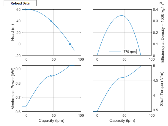
The reference brake power, W_brake,ref, is calculated as capacity·head/efficiency. The pump efficiency curve is quadratic with its peak corresponding to the Nominal brake power parameter, and it falls to zero when capacity is zero or maximum as the pump curve figure demonstrates.

The block calculates the reference capacity as:

$$q_{ref}=\frac{\dot{m}}{\rho }\frac{{\omega }_{ref}}{\omega }{\left(\frac{D_{ref}}{D}\right)}^3.$$

You can choose to be warned when the block flow rate becomes negative or exceeds the maximum pump capacity by setting Check if operating beyond normal pump operation to On.

1-D Tabulated Data Parameterization: Head and Brake Power as a Function of Capacity

When you set Pump parameterization to 1D tabulated data - head and brake power vs. capacity at reference shaft speed, the pressure gain over the pump functions with the Reference head vector parameter, ΔH_ref, which is a function of the reference capacity, q_ref:

$$\Delta p=\rho g\Delta H_{ref}(q_{ref}){\left(\frac{\omega }{{\omega }_{ref}}\right)}^2{\left(\frac{D}{D_{ref}}\right)}^2,$$

where g is the gravitational acceleration.

The block bases the shaft torque on the Reference brake power vector parameter, W_ref, which is a function of the reference capacity:

$$\tau =W_{ref}(q_{ref})\frac{{\omega }^2}{{\omega }_{ref}^3}\left(\frac{\rho }{{\rho }_{ref}}\right){\left(\frac{D}{D_{ref}}\right)}^5,$$

where ρ_ref is the Reference density parameter. The reference capacity is:

$$q_{ref}=\frac{\dot{m}}{\rho }\left(\frac{{\omega }_{ref}}{\omega }\right){\left(\frac{D_{ref}}{D}\right)}^3,$$

which the block uses to interpolate the values of the Reference capacity vector, Reference head vector, and Reference brake power vector parameters as a function of q_ref.

When the simulation is outside the range of the provided tables, the block extrapolates head based on the average slope of the pump curves and brake power to the nearest point.

2-D Tabulated Data Parameterization: Head and Brake Power as a Function of Capacity and Shaft Speed

When you set Pump parameterization to 2D tabulated data - head and brake power vs. capacity and shaft speed, the pressure gain over the pump is a function of the Head table, H(q,w) parameter, ΔH_ref, which is a function of the reference capacity, q_ref, and the shaft speed, ω:

$$\Delta p=\rho g\Delta H_{ref}(q_{ref},\omega ){\left(\frac{D}{D_{ref}}\right)}^2.$$

The shaft torque is a function of the Brake power table, Wb(q,w) parameter, W_ref, which is a function of the reference capacity, q_ref, and the shaft speed, ω:

$$\tau =\frac{W_{ref}(q_{ref},\omega )}{\omega }\left(\frac{\rho }{{\rho }_{ref}}\right){\left(\frac{D}{D_{ref}}\right)}^5.$$

The reference capacity is:

$$q_{ref}=\frac{\dot{m}}{\rho }{\left(\frac{D_{ref}}{D}\right)}^3.$$

When the simulation is outside the range of the provided tables, the block extrapolates head based on the average slope of the pump curves and brake power to the nearest point.

Missing Data

If your table has unknown data points, use NaN in place of these values. The block fills in the NaN elements by extrapolating based on the average slope of the pump curves. Do not use artificial numerical values because these values distort pump behavior when operating in that region. When using unknown data:

• The NaN elements in the table must be contiguous.

• The positions of the NaN elements in the Head table, H(q,w) and Brake power table, Wb(q,w) parameters must match each other.

• NaN elements must be located in the lower-left portion of the table, which corresponds to the highest capacity and lowest shaft speed.

Visualizing the Pump Curve

You can check the parameterized pump performance by plotting the head, power, efficiency, and torque as a function of the flow. To generate a plot of the current pump settings, in the block dialog box, click the Plot button next to Pump characteristics. When you modify the block parameters, refresh the data by clicking Reload Data in the figure window.

The default block parameterization results in these plots:

Assumptions and Limitations

• If the shaft rotates opposite to the specified mechanical orientation, pressure difference across the block drops to zero and the results may not be accurate.

• The block does not account for dynamic pressure in the pump. The block only considers pump head due to static pressure.

• Pre-defined parameterizations use available data and the block fills in missing data where necessary. Validate your model against expected results.

Examples

Lubrication System

A simplified version of a lubrication system fed with the centrifugal pump. The system consists of five major units: Pump Unit, Scavenge Unit, Heat Exchanger Manifold, Nozzle Manifold, and Control Unit. Both the pump and the scavenge unit are built around the centrifugal pump. The Scavenge Unit collects fluid discharged by nozzles and pumps it back into the reservoir of the Pump Unit. The Control Unit generates commands to bypass either the heat exchanger, represented as a local resistance, or the nozzles block. In a real system, these commands are generated by temperature sensors installed in lubrication cavities.

• Open Model

Water Supply System

A water supply system consisting of three pumping stations.

• Open Model

Ports

Conserving

A — Pump inlet

isothermal liquid

Isothermal liquid conserving port associated with the fluid inlet.

B — Pump outlet

isothermal liquid

Thermal liquid conserving port associated with the fluid outlet.

R — Impeller shaft

mechanical rotational

Mechanical rotational conserving port associated with the shaft.

C — Pump casing

mechanical rotational

Mechanical rotational conserving port associated with the case.

Parameters

Part Repository

Part selection — Open Block Parameterization Manager

button

Use the Select part button to open the Block Parameterization Manager tool and view the available parts.

Active part — Active part

part ID

Active part associated with the block.

Dependencies

To enable this parameter, apply a part to the block by using the Block Parameterization Manager.

Status — Restore default part parameters

button

Click the Restore parameters button to restore the parameterization to the active part. The name of the parameter is Status: unmodified if the part uses the default properties for the parameter, and Status: modified if the parameters have been modified from the associated active part.

Dependencies

To enable this parameter, apply a part to the block by using the Block Parameterization Manager.

Manage — Clear part association

button

Use the Clear part association button to clear the active part associated with the block.

Dependencies

To enable this parameter, apply a part to the block by using the Block Parameterization Manager.

Parameters

Pump parameterization — Head and brake power parameterization

Capacity, head, and brake power at reference shaft speed (default) | 1D tabulated data - head and brake power vs. capacity at reference shaft speed | 2D tabulated data - head and brake power vs. capacity and shaft speed

Parameterization of the pump head and brake power, specified as:

• Capacity, head, and brake power at reference shaft speed: Parameterize pump pressure gain and shaft torque with an analytical formula.

• 1D tabulated data - head and brake power vs. capacity at reference shaft speed: Parameterize head and brake power from tabulated data of the head and brake power at a given capacity.

• 2D tabulated data - head and brake power vs. capacity and shaft speed: Parameterize head and brake power from tabulated data of the head and brake power at a given capacity and shaft speed.

Nominal capacity — Pump volumetric flow rate

45 lpm (default) | positive scalar

Nominal pump volumetric flow rate at a reference shaft angular velocity.

Dependencies

To enable this parameter, set Pump parameterization to Capacity, head, and brake power at reference shaft speed.

Nominal head — Pump head

40 m (default) | positive scalar

Nominal pump pressure differential, normalized by gravity and the fluid density, at a reference shaft angular velocity.

Dependencies

To enable this parameter, set Pump parameterization to Capacity, head, and brake power at reference shaft speed.

Nominal brake power — Pump power

0.85 kW (default) | positive scalar

Nominal mechanical shaft power at a reference angular velocity.

Dependencies

To enable this parameter, set Pump parameterization to Capacity, head, and brake power at reference shaft speed.

Maximum head at zero capacity — Maximum pump head with no flow

60 m (default) | positive scalar

Maximum pump head with no flow at a reference angular velocity. This parameter determines the reference pressure differential over the pump, which the block uses to fit a quadratic equation for pressure in addition to the Nominal capacity, Nominal head, and Maximum capacity at zero head parameters.

Dependencies

To enable this parameter, set Pump parameterization to Capacity, head, and brake power at reference shaft speed.

Maximum capacity at zero head — Maximum flow rate with zero head

80 lpm (default) | positive scalar

Maximum fluid load with zero head at a reference angular velocity. This parameter determines the reference pressure differential over the pump, which the block uses to fit a quadratic equation for pressure in addition to the Nominal capacity, Nominal head, and Maximum head at zero capacity parameters.

Dependencies

To enable this parameter, set Pump parameterization to Capacity, head, and brake power at reference shaft speed.

Reference shaft speed — Reference shaft angular velocity for affinity law calculations

1770 rpm | 3500 rpm | positive scalar

Reference angular velocity for affinity law calculations. The default value depends on the Pump parameterization setting.

Dependencies

To enable this parameter, set Pump parameterization to either:

• Capacity, head, and brake power at reference shaft speed.

• 1D tabulated data - head and brake power vs. capacity at reference shaft speed.

Minimum shaft speed threshold as fraction of reference — Threshold for minimum shaft speed

1e-2 (default) | positive scalar

Threshold for the minimum shaft speed as a fraction of the reference shaft speed. The block uses this value to prevent the shaft speed from becoming zero and causing a division by zero error in the expression for q_ref.

Dependencies

To enable this parameter, set Pump parameterization to Capacity, head, and break power at reference shaft speed or 1D tabulated data – head and break power vs. capacity at reference shaft speed.

Reference capacity vector — Volumetric flow rate

[16.67, 30, 40, 53.33, 66.67, 83.33] lpm (default) | vector

Vector of volumetric flow rates for the tabular parameterization of the pump head or brake power. The elements in this vector correspond one-to-one with the elements in the Reference head vector and Reference brake power vector parameters. In normal operating conditions the elements in this parameter are nonnegative, but the block does accept negative values. Negative capacity is a non-normal operating condition that may arise from certain situations.

Dependencies

To enable this parameter, set Pump parameterization to 1D tabulated data - head and brake power vs. capacity at reference shaft speed.

Reference head vector — Pump head vector

[50, 47.5, 45, 40, 35, 25] m (default) | vector

Vector of the pump head values for the 1-D tabular parameterization of the pump head and brake power. This parameter corresponds one-to-one with the Reference capacity vector parameter. In normal operating conditions the elements in this parameter are nonnegative, but the block does accept negative values. Negative head, or pressure drop, is possible in non-normal operating conditions at the end of the vector.

Dependencies

To enable this parameter, set Pump parameterization to 1D tabulated data - head and brake power vs. capacity at reference shaft speed.

Reference brake power vector — Pump brake power vector

[.6, .75, .85, .93, .98, .99] kW (default) | vector

Vector of pump brake power values for the 1-D tabular parameterization of the pump head and brake power. This parameter corresponds one-to-one with the Reference capacity vector parameter. In normal operating conditions, the elements in this parameter are nonnegative, but the block does accept negative values. Negative brake power is possible in non-normal operating conditions at the end of the vector.

Dependencies

To enable this parameter, set Pump parameterization to 1D tabulated data - head and brake power vs. capacity at reference shaft speed.

Capacity vector, q — Volumetric displacement vector

[16.67, 23.33, 30, 40, 53.33, 60] lpm (default) | vector

Vector of volumetric flow rates for the tabular parameterization of the pump head. This vector forms an independent axis with the Shaft speed vector, w parameter for the 2-D Head table, H (q,w) and Brake power table, Wb(q,w) parameters. The vector elements must be listed in ascending order. In normal operating conditions, the elements in this parameter are nonnegative, but the block does accept negative values. Negative capacity is a non-normal operating condition that may arise from certain situations.

Dependencies

To enable this parameter, set Pump parameterization to 2D tabulated data - head and brake power vs. capacity and shaft speed.

Shaft speed vector, w — Angular velocity vector

[2450, 2800, 3150, 3500] rpm (default) | vector

Vector of shaft angular velocity values for the tabular parameterization of the pump head. This vector forms an independent axis with the Capacity vector, q parameter for the 2-D Head table, H (q,w) and Brake power table, Wb(q,w) parameters. The vector elements must be listed in ascending order and must be greater than 0.

Dependencies

To enable this parameter, set Pump parameterization to 2D tabulated data - head and brake power vs. capacity and shaft speed.

Head table, H(q,w) — Pump head matrix

[25, 32.7, 42.5, 50; 24, 31.7, 41, 49; 22.7, 30.5, 39, 47.5; 20, 28, 36, 45; 15.7, 24, 32, 40; 12.5, 21, 29.5, 37.5] m (default) | M-by-N matrix

M-by-N matrix of pump head values at the specified volumetric flow rate and angular velocity. In normal operating conditions, the elements in this parameter are nonnegative, but the block does accept negative values. Negative head, or pressure drop, is possible in non-normal operating conditions at the bottom of the table. The block employs linear interpolation between the table elements. M and N are the sizes of the corresponding vectors:

• M is the number of elements in the Capacity vector, q parameter.

• N is the number of elements in the Shaft speed vector, w parameter. All rows must be in strictly ascending order.

If your table has unknown data points, use NaN in place of these values. The block fills in the NaN elements by extrapolating based on the average slope of the pump curves. Do not use artificial numerical values because these values distort pump behavior when operating in that region. When using unknown data:

• The NaN elements in the table must be contiguous.

• The positions of the NaN elements in the Head table, H(q,w) and Brake power table, Wb(q,w) parameters must match each other.

• NaN elements must be located in the lower-left portion of the table, which corresponds to the highest capacity and lowest shaft speed.

Dependencies

To enable this parameter, set Pump parameterization to 2D tabulated data - head and brake power vs. capacity and shaft speed.

Brake power table, Wb(q,w) — Pump brake power matrix

[.28, .38, .5, .6; .31, .41, .55, .68; .33, .44, .6, .75; .36, .48, .65, .83; .38, .53, .72, .93; .39, .55, .75, .97] kW (default) | M-by-N matrix

M-by-N matrix of pump brake power values at the specified volumetric flow rate and angular velocity. In normal operating conditions these values are nonnegative, but the block does accept negative values. The block employs linear interpolation between the table elements. M and N are the sizes of the corresponding vectors:

• M is the number of vector elements in the Capacity vector, q parameter.

• N is the number of vector elements in the Shaft speed vector, w parameter. All rows must be in strictly ascending order.

If your table has unknown data points, use NaN in place of these values. The block fills in the NaN elements by extrapolating based on the average slope of the pump curves. Do not use artificial numerical values because these values distort pump behavior when operating in that region. When using unknown data:

• The NaN elements in the table must be contiguous.

• The positions of the NaN elements in the Head table, H(q,w) and Brake power table, Wb(q,w) parameters must match each other.

• NaN elements must be located in the lower-left portion of the table, which corresponds to the highest capacity and lowest shaft speed.

Dependencies

To enable this parameter, set Pump parameterization to 2D tabulated data - head and brake power vs. capacity and shaft speed.

Reference density — Fluid density for given pump performance data

998 kg/m^3 (default) | positive scalar

Reference fluid density. The reference or data sheet typically specifies this value. This parameter scales the pump performance between different fluids.

Dependencies

To enable this parameter, set Pump parameterization to 1D tabulated data - head and brake power vs. capacity at reference shaft speed or 2D tabulated data - head and brake power vs. capacity and shaft speed.

Impeller diameter scale factor — Ratio of model diameter to reference diameter for affinity law calculations

1 (default) | positive scalar

Ratio of the model-to-reference diameter for affinity law calculations. Modify this value if there is a difference between your reference and the system impeller diameters, such as when testing pump scaling. For system pumps smaller than the reference pump, use a value less than one. For system pumps larger than the reference pump, use a value greater than one. The block does not reflect changes in pump efficiency due to pump size.

Mechanical orientation — Shaft normal rotational direction

Positive angular velocity of port R relative to port C corresponds to normal pump operation (default) | Negative angular velocity of port R relative to port C corresponds to normal pump operation

Shaft rotational direction for flow from port A to B.

Check if operating beyond normal pump operation — Option to notify when block is beyond operating bounds

None (default) | Warning | Error

Option to notify if the block operates outside of the normal pump boundary. This situation occurs when the flow rate through the pump is negative or beyond the maximum capacity of the pump.

Dependencies

To enable this parameter, set Pump parameterization to Capacity, head, and brake power at reference shaft speed.

Plots

Pump characteristics — Generate pump characteristics plot

button

Use the Plot button to generate the pump characteristics plot.

Extended Capabilities

C/C++ Code Generation
Generate C and C++ code using Simulink® Coder™.

Version History

Introduced in R2020a

R2023a: Expose threshold for low shaft speed

Use the Minimum shaft speed threshold as fraction of reference parameter to control the minimum shaft speed threshold as a fraction of the reference shaft speed. The Minimum shaft speed threshold as fraction of reference parameter is available in the block when the Pump parameterization parameter is Capacity, head, and break power at reference shaft speed or 1D tabulated data – head and break power vs. capacity at reference shaft speed.

R2022b: Extend performance beyond normal operating conditions

Both the 1-D and 2-D parameterizations now allow negative values. When simulation is outside the range of the provided table, the block extrapolates the pump head based on the average slope of the pump curves.

You can now use NaN elements where pump data is unavailable. These 2-D tabulated parameters support contiguous NaN elements in the lower-left portion of the table:

• Head table H(q,w)

• Brake power table, Wb(q,w)

For each block, if the shaft rotates opposite to the specified mechanical orientation, the pressure difference across the block drops to zero and the results may not be accurate.