Estimate State-Space Models in System Identification App

R2026b

Prerequisites

Import data into the System Identification app. See Represent Data. For supported data formats, see Data Supported by State-Space Models.
Perform data preprocessing. To improve the accuracy of your model, you detrend your data. See Data Preparation.

Select Estimate > State Space Models.
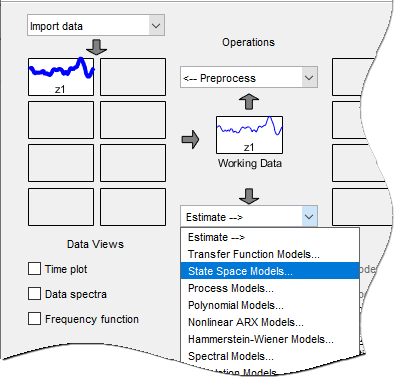
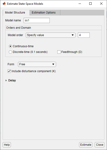
The State Space Models dialog box opens.
Tip
For more information on the options in the dialog box, click Help.
Model name displays the default model name. To change the name, enter a new name. The name of the model must be unique in the Model Board.
Select the Specify value option (if not already selected) and specify the model order in the edit field. Model order refers to the number of states in the state-space model.
Tip
When you do not know the model order, search for and select an order. For more information, see Estimate Model with Selected Order in the App.
Select the Continuous-time or Discrete-time option to specify the type of model to estimate.
You cannot estimate a discrete-time model if the working data is continuous-time frequency-domain data.
Specify the elements to include in the model structure, including feedthrough (D matrix) and the disturbance component (K matrix.) Specify the model form, such as canonical form, by selecting from the options in Form. To specify delays, expand the Delay section.

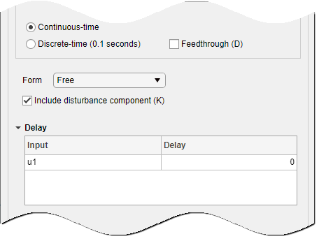
For more information about the type of state-space parameterization, see Supported State-Space Parameterizations.
Select the Estimation Options tab to select the estimation method and configure the cost function.
Select one of the methods in Estimation method and configure the options. For more information about these methods, see State-Space Model Estimation Methods.
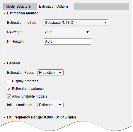
In the N4Weight drop-down list, specify the weighting scheme used for singular-value decomposition by the N4SID algorithm.
The N4SID algorithm is used both by the subspace and Prediction Error Minimization (PEM) methods.
In the N4Horizon field, specify the forward and backward prediction horizons used by the N4SID algorithm.
In the Estimation Focus drop-down list, select whether to optimize the estimation for one-step-ahead prediction or for simulation. For more information about these options, options see Assigning Estimation Weightings.
Select the Allow unstable models check box to specify whether to allow the estimation process to use parameter values that may lead to unstable models.
This option is available only when Estimation Focus is Prediction. An unstable model is delivered only if it produces a better fit to the data than other stable models computed during the estimation process.
Select the Estimate covariance check box if you want the algorithm to compute parameter uncertainties.
Effects of such uncertainties are displayed on plots as model confidence regions. Skipping uncertainty computation reduces computation time for complex models and large data sets.
Select the Display progress check box to open a progress viewer window during estimation.
In the Initial conditions list, specify how you want the algorithm to treat initial states. For more information about the available options, see Specifying Initial States for Iterative Estimation Algorithms.
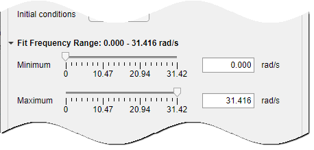
If you want to limit the estimation process to a specific frequency range, expand Fit Frequency Range. Create a passband filter by specifying the minimum and maximum passband frequencies.
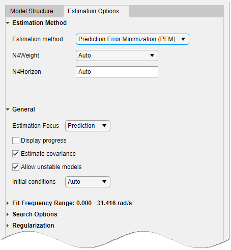
In the N4Weight drop-down list, specify the weighting scheme used for singular-value decomposition by the N4SID algorithm.
The N4SID algorithm is used both by the subspace and Prediction Error Minimization (PEM) methods.
In the N4Horizon field, specify the forward and backward prediction horizons used by the N4SID algorithm.
In the Estimation Focus drop-down list, select whether to optimize the estimation for one-step-ahead prediction or for simulation. For more information about these options, options see Assigning Estimation Weightings.
Select the Allow unstable models check box to specify whether to allow the estimation process to use parameter values that may lead to unstable models.
This option is available only when Estimation Focus is Prediction. An unstable model is delivered only if it produces a better fit to the data than other stable models computed during the estimation process.
Select the Estimate covariance check box if you want the algorithm to compute parameter uncertainties.
Effects of such uncertainties are displayed on plots as model confidence regions. Skipping uncertainty computation reduces computation time for complex models and large data sets.
Select the Display progress check box to open a progress viewer window during estimation.
In Initial conditions, specify how you want the algorithm to treat initial states. For more information about the available options, see Specifying Initial States for Iterative Estimation Algorithms.
If you want to limit the estimation process to a specific frequency range, expand Fit Frequency Range. Create a passband filter by specifying the minimum and maximum passband frequencies.
Expand Search Options to specify options for controlling the search iterations.
In the Search Options section of Estimation Options, you can specify the following options:
Search method — Method used by the iterative search algorithm. Search method is auto by default. Search methods include Gauss-Newton(gn), Adaptive Gauss-Newton(gna), Levenberg-Marquardt(lm), Trust-Region Reflective Newton (lsqnonlin), Gradient Search (grad), Sequential Quadratic Programming (fmincon:sqp), or Interior Point (fmincon: interior-point). The descent direction is calculated successively at each iteration until a sufficient reduction in error is achieved.
Output weight — Weighting applied to the loss function to be minimized. Use this option for multi-output estimations only. Specify as 'noise' or a positive semidefinite matrix of size equal the number of outputs.
Maximum iterations — Maximum number of iterations to use during search.
Tolerance — Tolerance value when the iterations should terminate.
Outlier threshold — Robustification of the quadratic criterion of fit.
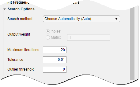
Expand Regularization to obtain regularized estimates of model parameters. Specify the regularization constants Lambda and R.

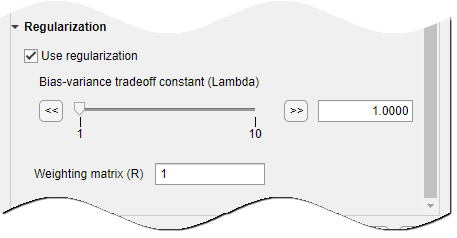
To learn more about regularization, see Regularized Estimates of Model Parameters.
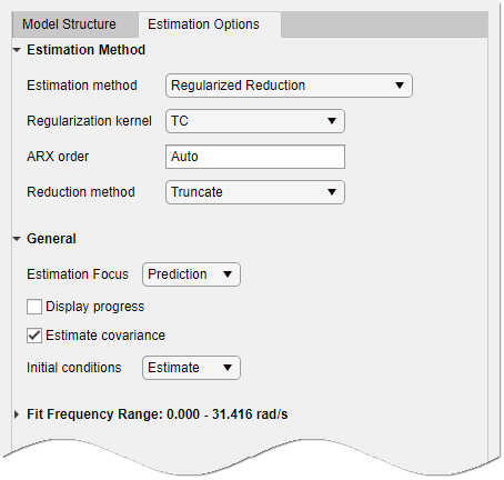
In the Regularization Kernel drop-down list, select the regularizing kernel to use for regularized estimation of the underlying ARX model. To learn more, see Regularized Estimates of Model Parameters.
In the ARX Orders field, specify the order of the underlying ARX model. By default, the orders are automatically computed by the estimation algorithm. If you specify a value, it is recommended that you use a large value for nb order. To learn more about ARX orders, see arx.
In the Estimation Focus drop-down list, select whether to optimize the estimation for one-step-ahead prediction or for simulation. For more information about these options, options see Assigning Estimation Weightings.
In the Reduction Method drop-down list, specify the reduction method:
Truncate — Discards the specified states without altering the remaining states. This method tends to product a better approximation in the frequency domain, but the DC gains are not guaranteed to match.
MatchDC — Discards the specified states and alters the remaining states to preserve the DC gain.
Select the Estimate covariance check box if you want the algorithm to compute parameter uncertainties.
Effects of such uncertainties are displayed on plots as model confidence regions. Skipping uncertainty computation reduces computation time for complex models and large data sets.
Select the Display progress check box to open a progress viewer window during estimation.
In Initial conditions, specify how you want the algorithm to treat initial states. For more information about the available options, see Specifying Initial States for Iterative Estimation Algorithms.
If you want to limit the estimation process to a specific frequency range, expand Fit Frequency Range. Create a passband filter by specifying the minimum and maximum passband frequencies.
This estimation process uses parameter values that always lead to a stable model.
Click Estimate to estimate the model. A new model gets added to the System Identification app.

Next Steps

Validate the model by selecting the appropriate response type in the Model Views area of the app. For more information about validating models, see Validating Models After Estimation.
Export the model to the MATLAB^® workspace for further analysis by dragging it to the To Workspace rectangle in the app.

Assigning Estimation Weightings

You can specify both how the estimation algorithm weights the fit at various frequencies and what frequency range the app uses. In the app, set Estimation Focus to one of the following options:

Prediction — Uses the ratio of the input spectrum U to the inverse of the noise model H to weight the relative importance of data across the full frequency range. This weighting corresponds to minimizing one-step-ahead prediction, which typically favors the fit over a short time interval. Optimized for output prediction applications.
Simulation — Uses the input spectrum only, and not the noise model, for weighting. Optimized for output simulation applications.

You can apply a passband to limit the frequency range over which the estimation algorithm performs the fit.

For more information on estimation weighting, see the section Effects of Focus and WeightingFilter Options in Loss Function and Model Quality Metrics.