Fast Fourier Transform
An image is a 2-D signal where the image intensity is dependent on 2-D spatial variables. In the context of a 2-D image, frequency refers to the rate at which pixel intensity values change spatially across the image.
Just as you can represent 1-D signals as a sum of 1-D complex exponentials of different magnitudes, frequencies, and phases, you can represent 2-D signals, such as images, as a sum of 2-D complex exponentials of different magnitudes, frequencies, and phases. The magnitude and phase of each frequency comprises the frequency-domain representation of the image. The magnitude and phase of each frequency component indicates how much of that frequency is present in the image. The frequency-domain representation of an image plays a critical role in a broad range of image processing applications.
Image Analysis — The magnitude and phase of each frequency component indicates how much of that frequency is present in the image, enabling you to better understand the image.
Image Filtering — You can use frequency-based filtering to enhance or suppress certain features. For example, a high-pass filter can emphasize edges by removing low-frequency components, while a low-pass filter can smooth an image by removing high-frequency noise.
Image Compression — Techniques like JPEG compression use frequency analysis to reduce image size by discarding less critical high-frequency information.
Image Reconstruction — You can use frequency information to reconstruct images from incomplete data.
The Fourier transform is a widely used method for transforming a spatial-domain image into its frequency-domain representation.
Discrete Fourier Transform (DFT)
The Fourier transform is a representation of a signal as a sum of complex exponentials of varying magnitudes, frequencies, and phases. Digital images are spatially discrete signals. Computing the Fourier transform at equally spaced discrete frequencies makes it convenient to process in digital systems. The Fourier transform, when computed at equally spaced discrete frequencies, is called the discrete Fourier transform (DFT). The fast Fourier transform (FFT) is an algorithm to quickly compute the DFT.
The DFT is defined for a discrete 2-D function f(m,n) that is nonzero only over the finite region and , such as for an image of size M-by-N. The 2-D M-by-N DFT and inverse M-by-N DFT relationships are given by:
and
The values F(p,q) are the DFT coefficients of f(m,n). The DFT coefficients F(p,q) represent the Fourier transform of the image at the discrete frequencies (2πp/M,2πq/N), where each coefficient represents the strength of the 2-D frequency pair (2πp/M,2πq/N). F(0,0) is the constant component, or zero-frequency component, of the Fourier transform, which indicates the average intensity level of the image. Note that matrix indices in MATLAB® always start at 1 rather than 0, which means the matrix elements f(1,1) and F(1,1) correspond to the mathematical quantities f(0,0) and F(0,0), respectively. The inverse DFT equation means that you can represent f(m,n) as a sum of complex exponentials with different frequencies.
The fft, fft2, and fftn functions implement the fast
Fourier transform algorithm for computing the 1-D DFT, 2-D DFT, and N-D DFT,
respectively. The ifft, ifft2, and ifftn functions compute the inverse
DFT.
Interpret Fourier Transform of Images
High spatial frequency in an image represents rapid changes in image intensity, such as edges, fine details, and textures. High-frequency components are crucial for defining sharpness and detail in an image, and are essential for the clarity and detail of the image. Low spatial frequency in an image represents slow changes in image intensity, such as smooth variations in intensity and color. Low-frequency components represent the general shape and structure of the image and are critical for the overall appearance and context of the image.
Consider an image f(m,n) that has intensity equal to 1 within a rectangular region and 0 everywhere else. You can create a 2-D matrix representing the image.
f = zeros(30,30);
f(5:24,13:17) = 1;
imshow(f)

You can compute and visualize the DFT of the image f.
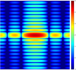
Visualizing the logarithm of the DFT magnitude, especially if the range of the DFT
coefficient magnitudes is significantly skewed, can be more informative than
visualizing their explicit values. Because the DFT is periodic, visualizations
typically display it over a single period. Observe that the DFT has more magnitude
at high horizontal frequencies than at high vertical frequencies. This reflects the
fact that horizontal cross-sections of the image have higher frequency content
because of faster transitions in image intensity as compared to vertical
cross-sections of the image.
F = fft2(f);
absF = abs(F);
logabsF = log(absF);
imshow(logabsF,[-1 5]);
colormap(jet)
colorbar

You can obtain a finer frequency representation by computing the DFT at more frequencies.
F = fft2(f,256,256);
absF = abs(F);
logabsF = log(absF);
imshow(logabsF,[-1 5]);
colormap(jet)
colorbar

Although the zero-frequency coefficient is the peak of the
magnitude spectrum, the visualization displays the zero-frequency coefficient in the
corner rather than the center. You can fix this problem by using the fftshift function, which swaps the
quadrants of F so that the zero-frequency coefficient is in the
center.
F = fft2(f,256,256);
F = fftshift(F);
absF = abs(F);
logabsF = log(abs(F));
imshow(logabsF,[-1 5]);
colormap(jet)
colorbar
Examples of Discrete Fourier Transforms of Simple Shapes
| Image | Fourier Transform (Log Magnitude) | Interpretation |
|---|---|---|
|
|
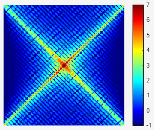
| The image has a narrow pulse in cross-sections taken at 45 degrees angle relative to horizontal. Thus high frequencies in the 45 degree direction have a high magnitude. The image has a broad pulse in cross-sections taken at -45 degrees angle relative to horizontal. Thus high frequencies in the -45 degree direction have a low magnitude. |
|
|
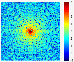
| The image is isotropic, with similar intensity transition in all directions. Thus, the magnitude of frequencies is similar in all directions. |
|
|
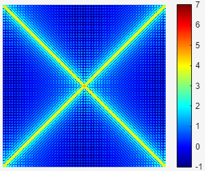
| The sharpest intensity transitions in the image are along the diagonals. Thus, the magnitude of high frequencies is higher along the diagonals. |


Applications of Fourier Transform
If you modify an image, its DFT changes. Similarly, if you modify the DFT of an image, and then compute the inverse DFT, the output image is a modified version of the input image. When modifying an image, you can choose to make the required modifications in the spatial domain or the corresponding frequency-domain modifications in the frequency domain. For example, you can make these modifications to an image by performing corresponding operations on its DFT.
If you retain low-frequency components and attenuate or remove high-frequency components in the DFT, the image becomes smoother, as you reduce fine details and noise (which are high-frequency components). This is useful for image denoising and blurring the image.
If you retain high-frequency components and attenuate or remove low-frequency components in the DFT, the image appears sharper, with enhanced edges and fine details. This is useful for edge detection and highlighting features.
If you selectively retain, remove, or emphasize specific frequency components or specific bands of frequencies, you can isolate, suppress, or highlight specific patterns or textures in the image.
If you discard high-frequency components, you can reduce the image size with minimal loss of perceived quality, as the human eye is less sensitive to high-frequency details. This is a principle used in image compression.
A key property of the Fourier transform is that the multiplication of two Fourier transforms corresponds to the convolution of the associated spatial functions. This property, together with the fast Fourier transform, forms the basis for a fast convolution algorithm. The DFT of the impulse response of a linear filter gives the frequency response of the filter. You can perform FFT-based image filtering by performing these steps.
Zero-pad the linear filter to the size of the image.
Compute the frequency response of the zero-padded linear filter using FFT.
Compute the FFT of the image.
Multiply the FFT of the image with the frequency response of the linear filter.
Compute the inverse FFT of the product to get the filtered output.
[M,N] = size(image);
fft_image = fft2(image);
fft_filter = fft2(filter,M,N);
fft_filteredImage = fft_image.*fft_filter;
filteredImage = ifft2(fft_filteredImage);
The FFT-based convolution method is most effective when used for large inputs. For
small inputs, convolution in spatial domain is generally faster. You can use the
imfilter function for both large
and small inputs, because it automatically decides whether to perform the
convolution in the frequency domain or in the spatial domain.
The freqz2 function calculates and
displays the frequency response of a filter. The frequency response of the Gaussian
convolution kernel shows that this filter passes low frequencies and attenuates high
frequencies, whereas the frequency response of the Laplacian convolution kernel
shows that this filter passes high frequencies and attenuates low frequencies. See
Design Linear Image Filters in the Frequency Domain for more information
about linear filtering, filter design, and frequency responses.
h = fspecial("gaussian");
freqz2(h)
h = fspecial("laplacian");
freqz2(h)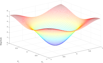
See Also
fft2 | fftn | ifft2 | ifftn | fftshift | ifftshift | freqz2