imnlmfilt

Non-local means filtering of image

Syntax

J = imnlmfilt(I)

J = imnlmfilt(I,Name,Value)

[J,estDoS] = imnlmfilt(___)

Description

J = imnlmfilt(I) applies a non-local means-based filter to the grayscale or color image I and returns the resulting image in J.

J = imnlmfilt(I,Name,Value) uses name-value pairs to change the behavior of the non-local means filter.

[J,estDoS] = imnlmfilt(___) also returns the degree of smoothing, estDoS, used to estimate the denoised pixel value.

Examples

Denoise Grayscale Image Using Non-Local Means Filter

Read a grayscale image.

I = imread('cameraman.tif');

Add zero-mean white Gaussian noise with 0.0015 variance to the image using the imnoise function.

noisyImage = imnoise(I,'gaussian',0,0.0015);

Remove noise from the image through non-local means filtering. The imnlmfilt function estimates the degree of smoothing based on the standard deviation of noise in the image.

[filteredImage,estDoS] = imnlmfilt(noisyImage);

Display the noisy image (left) and the non-local means filtered image (right) as a montage. Display the estimated degree of smoothing, estDoS, in the figure title.

The non-local means filter removes noise from the input image but preserves the sharpness of strong edges, such as the silhouette of the man and buildings. This function also smooths textured regions, such as the grass in the foreground of the image, resulting in less detail when compared to the noisy image.

montage({noisyImage,filteredImage})
title(['Estimated Degree of Smoothing, ', 'estDoS = ',num2str(estDoS)])

Denoise Color Image Using Non-Local Means Filter

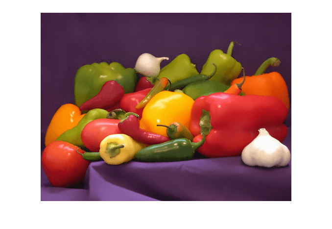
Read a color image.

imRGB = imread('peppers.png');

Add white Gaussian noise with zero mean and 0.0015 variance to the image using the imnoise function. Display the noisy RGB image.

noisyRGB = imnoise(imRGB,'gaussian',0,0.0015);
imshow(noisyRGB)

Convert the noisy RGB image to the L*a*b color space, so that the non-local means filter smooths perceptually similar colors.

noisyLAB = rgb2lab(noisyRGB);

Extract a homogeneous L*a*b patch from the noisy background to compute the noise standard deviation.

roi = [210,24,52,41];
patch = imcrop(noisyLAB,roi);

In this L*a*b patch, compute the Euclidean distance from the origin, edist. Then, calculate the standard deviation of edist to estimate the noise.

patchSq = patch.^2;
edist = sqrt(sum(patchSq,3));
patchSigma = sqrt(var(edist(:)));

Set the 'DegreeOfSmoothing' value to be higher than the standard deviation of the patch. Filter the noisy L*a*b* image using non-local means filtering.

DoS = 1.5*patchSigma;
denoisedLAB = imnlmfilt(noisyLAB,'DegreeOfSmoothing',DoS);

Convert the filtered L*a*b image to the RGB color space. Display the filtered RGB image.

denoisedRGB = lab2rgb(denoisedLAB,'Out','uint8');
imshow(denoisedRGB)

Compare a patch from the noisy RGB image (left) and the same patch from the non-local means filtered RGB image (right).

roi2 = [178,68,110,110];
montage({imcrop(noisyRGB,roi2),imcrop(denoisedRGB,roi2)})

Input Arguments

I — Image to filter

2-D grayscale image | 2-D color image

Image to filter, specified as a 2-D grayscale image of size m-by-n or a 2-D color image of size m-by-n-by-3. The size of I must be greater than or equal to 21-by-21.

Data Types: single | double | int8 | int16 | int32 | uint8 | uint16 | uint32

Name-Value Arguments

Specify optional pairs of arguments as Name1=Value1,...,NameN=ValueN, where Name is the argument name and Value is the corresponding value. Name-value arguments must appear after other arguments, but the order of the pairs does not matter.

Before R2021a, use commas to separate each name and value, and enclose Name in quotes.

Example: J = imnlmfilt(I,'DegreeOfSmoothing',10);

DegreeOfSmoothing — Degree of smoothing

positive number

Degree of smoothing, specified as the comma-separated pair consisting of 'DegreeOfSmoothing' and a positive number. As this value increases, the smoothing in the resulting image J increases. If you do not specify 'DegreeOfSmoothing', then the default value is the standard deviation of noise estimated from the image. For more information, see Default Degree of Smoothing.

SearchWindowSize — Search window size

21 (default) | odd-valued positive integer

Search window size, specified as the comma-separated pair consisting of 'SearchWindowSize' and an odd-valued positive integer, s. The search for similar neighborhoods to a pixel is limited to the s-by-s region surrounding that pixel. SearchWindowSize affects the performance linearly in terms of time. SearchWindowSize cannot be larger than the size of the input image, I.

ComparisonWindowSize — Comparison window size

5 (default) | odd-valued positive integer

Comparison window size, specified as the comma-separated pair consisting of 'ComparisonWindowSize' and an odd-valued positive integer, c. The imnlmfilt function computes similarity weights using the c-by-c neighborhood surrounding pixels. ComparisonWindowSize must be less than or equal to SearchWindowSize. For more information, see Estimate Denoised Pixel Value.

Output Arguments

J — Non-local means filtered image

2-D grayscale image | 2-D color image

Non-local means filtered image, returned as a 2-D grayscale image or 2-D color image of the same size and data type as the input image, I.

estDoS — Estimated degree of smoothing

positive number

Estimated degree of smoothing, returned as a positive number. If you specify DegreeOfSmoothing, then imnlmfilt returns the same value in estDoS. Otherwise, imnlmfilt returns the default degree of smoothing estimated using Default Degree of Smoothing.

Tips

• To smooth perceptually close colors in an RGB image, convert the image to the CIE L*a*b* color space using rgb2lab before applying the non-local means filter. To view the results, first convert the filtered L*a*b* image to the RGB color space using lab2rgb.

• If the data type of I is double, then computations are performed in data type double. Otherwise, computations are performed in data type single.

Algorithms

Default Degree of Smoothing

The default value of 'DegreeOfSmoothing' is the standard deviation of noise estimated from the image. To estimate the standard deviation, imnlmfilt convolves the image with a 3-by-3 filter proposed by J. Immerkær [2]. When I is a color image, the default value of 'DegreeOfSmoothing' is the standard deviations of noise averaged across the channels.

Estimate Denoised Pixel Value

The non-local means filtering algorithm estimates the denoised value of pixel p using these steps.

1. For a specific pixel, q, in the search window, calculate the weighted Euclidean distance between pixel values in the c-by-c comparison windows surrounding p and q. For color images, include all channels in the Euclidean distance calculation.

   The weight is a decreasing exponential function whose rate of decay is determined by the square of 'DegreeOfSmoothing'. When an image is noisy, 'DegreeOfSmoothing' is large and all pixels contribute to the Euclidean distance calculation. When an image has little noise, 'DegreeOfSmoothing' is small and only pixels with similar values contribute to the Euclidean distance calculation.

   The result is a numeric scalar that indicates the similarity between the neighborhood of p and the neighborhood of q.

   Note

   In the implementation by A. Buades et al. [1], the Euclidean distance between two comparison windows is convolved with a Gaussian kernel of size c-by-c. This convolution gives more weight to the Euclidean distance between pixel values for pixels near the center of the comparison window. The imnlmfilt function omits this step for computational efficiency.

2. Repeat this computation for each of the other pixels in the s-by-s search window, finding the weighted Euclidean distance between pixel p and each of those pixels. The result is an s-by-s similarity matrix that indicates similarity between the neighborhood of p and the other neighborhoods in the search window.

3. Normalize the similarity matrix.

4. Using the weights in the normalized similarity matrix, compute the weighted average of pixel values in the s-by-s search window around pixel p. The result is the denoised value of p.

References

[1] Buades, A., B. Coll, and J.-M. Morel. "A Non-Local Algorithm for Image Denoising." 2005 IEEE^® Computer Society Conference on Computer Vision and Pattern Recognition. Vol. 2, June 2005, pp. 60–65.

[2] Immerkær, J. "Fast Noise Variance Estimation." Computer Vision and Image Understanding. Vol. 64, Number 2, Sept. 1996, pp. 300–302.

Extended Capabilities

Thread-Based Environment

Run code in the background using MATLAB® backgroundPool or accelerate code with Parallel Computing Toolbox™ ThreadPool.

This function fully supports thread-based environments. For more information, see Run MATLAB Functions in Thread-Based Environment.

Version History

Introduced in R2018b

R2022b: Support for thread-based environments

imnlmfilt now supports thread-based environments.