Main Content

pdeval

Interpolate numerical solution of PDE

Description

[u,dudx] = pdeval(m,xmesh,usol,xq) interpolates a numerical solution returned by pdepe at new query points xq, and returns the interpolated values of the solution u and their partial derivative dudx. The m, xmesh, and usol arguments are reused from a previous call to pdepe:

  • The numerical solution produced by sol = pdepe(m,@pdefun,@pdeic,@pdebc,xmesh,tspan) uses the coordinate symmetry m and spatial mesh xmesh to return a 3-D matrix of the solution values sol. Reuse the m and xmesh inputs used to calculate the solution when you call pdeval.

  • The input vector usol = sol(i,:,k) is the value of component k of the solution at time tspan(i). When there is only one solution component, usol is a row extracted from the solution matrix usol = sol(i,:).

example

Examples

collapse all

Use pdepe to solve a partial differential equation, and then use pdeval to evaluate the solution at additional points.

Solve PDE

Use pdepe to solve the pdex1 example problem. You can type edit pdex1 to see more details on the problem, or see pdepe for details on the PDE solution process. The required functions to solve the pdex1 problem are included at the end of this example as local functions.

m = 0;
x = linspace(0,1,20);
t = linspace(0,2,5);
sol = pdepe(m,@pdex1pde,@pdex1ic,@pdex1bc,x,t);

Interpolate Solution

The solution sol generated by pdepe uses 20 points for x, evenly spaced between 0 and 1. Create a vector of query points that are located midway between the points used by pdepe.

xq = x;
xq(1:end-1) = xq(1:end-1) + diff(xq)./2;

Use pdeval to interpolate the solution at the query points. Since there is only one solution component, you can extract a row from sol to operate on, such as sol(2,:).

[u,dudx] = pdeval(m,x,sol(2,:),xq);

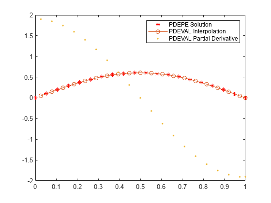
Plot the solution computed by pdepe, as well as the interpolated solution and its partial derivative computed by pdeval.

plot(x,sol(2,:),'r*')
hold on
plot(xq,u,'-o')
plot(xq,dudx,'.')
hold off
legend('PDEPE Solution', 'PDEVAL Interpolation', 'PDEVAL Partial Derivative')

Figure contains an axes object. The axes object contains 3 objects of type line. One or more of the lines displays its values using only markers These objects represent PDEPE Solution, PDEVAL Interpolation, PDEVAL Partial Derivative.

Local Functions

Listed here are the local helper functions that the PDE solver pdepe calls to calculate the solution.

function [c,f,s] = pdex1pde(x,t,u,DuDx)
c = pi^2;
f = DuDx;
s = 0;
end
% ------------------------------------------------------
function u0 = pdex1ic(x)
u0 = sin(pi*x);
end
% ------------------------------------------------------
function [pl,ql,pr,qr] = pdex1bc(xl,ul,xr,ur,t)
pl = ul;
ql = 0;
pr = pi * exp(-t);
qr = 1;
end

Input Arguments

collapse all

Coordinate symmetry used with pdepe, specified as one of the values in this table. Specify the same coordinate symmetry you used in the initial call to pdepe.

ValueSymmetry

0

Slab/Cartesian

1

Cylindrical

2

Spherical

Spatial mesh used with pdepe, specified as a vector [x0 x1 ... xn] containing the points at which a numerical solution was computed. Specify the same spatial mesh you used in the initial call to pdepe.

Data Types: single | double

Extracted solution component, specified as a vector of values computed by pdepe for one solution component at a particular time.

pdepe returns the solution in a 3-D array sol, where sol(i,j,k) approximates the kth component of the solution u k evaluated at time t(i) and spatial point xmesh(j). You can create the input usol with the command usol = sol(i,:,k), where sol(i,:,k) is the value of component k of the solution at time tspan(i), evaluated on the entire spatial mesh xmesh. When there is only one solution component, usol is a row extracted from the solution matrix usol = sol(i,:).

Example: usol = sol(10,:,2) extracts the second solution component calculated at time tspan(10).

Example: usol = sol(5,:) extracts the solution calculated at time tspan(5).

Data Types: single | double
Complex Number Support: Yes

Query points, specified as a scalar or vector of x-coordinates. The points specified in xq must lie within the interval [min(xmesh) max(xmesh)].

Typically, the points in xq are specified between the values in xmesh to enable pdeval to evaluate the solution produced by pdepe on a finer mesh.

Example: xq = linspace(0,1,100) specifies 100 evenly spaced query points between 0 and 1.

Data Types: single | double
Complex Number Support: Yes

Output Arguments

collapse all

Interpolated solution, returned as a vector with the same size as xq.

Partial derivative of interpolated solution, returned as a vector with the same size as xq.

Tips

  • pdeval evaluates the partial derivative ux rather than the flux f(x,t,u,ux). Although the flux is continuous, the partial derivative can have a jump at a material interface.

Extended Capabilities

Thread-Based Environment
Run code in the background using MATLAB® backgroundPool or accelerate code with Parallel Computing Toolbox™ ThreadPool.

Version History

Introduced before R2006a