Accelerate Brain MRI Segmentation Using GPU

Since R2026a

This example shows how to accelerate segmentation of a brain MRI using a deep neural network on a GPU.

A neural network can often segment image data faster on a GPU than on a CPU. It can also be faster to pre- and postprocess the image data on a GPU. Starting from the code in the Brain MRI Segmentation Using Pretrained 3-D U-Net Network example, this example demonstrates how to speed up processing and segmenting 3-D images by modifying your code to run on a GPU. You can use a similar approach to accelerate other medical imaging workflows.

Check GPU Support

GPU acceleration in MATLAB® requires Parallel Computing Toolbox™ and a supported GPU device. For information on supported devices, see GPU Computing Requirements (Parallel Computing Toolbox).

Check whether you have a supported GPU.

gpu = gpuDevice;
disp(gpu.Name + " GPU selected.")

NVIDIA RTX A5000 GPU selected.

If a function supports GPU array input, that support is listing in the Extended Capabilities section of its documentation page. You can also filter lists of functions in the documentation to show only functions that support GPU acceleration. For more information, see Run MATLAB Functions on a GPU (Parallel Computing Toolbox).

After checking that you have a supported GPU, follow the steps in this example. These are the same steps as in the original example, but with minor modifications to send data to the GPU and run functions on the GPU where possible. The code requires very little modification to run on a GPU.

Download Brain MRI and Label Data

This example uses a subset of the CANDI data set [2] [3]. The subset consists of a brain MRI volume and the corresponding ground truth label volume for one patient. Both files are in the NIfTI file format. The total size of the data files is ~2.5 MB.

Run this code to download the dataset from the MathWorks® website and unzip the downloaded folder.

zipFile = matlab.internal.examples.downloadSupportFile("image","data/brainSegData.zip");
filepath = fileparts(zipFile);
unzip(zipFile,filepath)

The dataDir folder contains the downloaded and unzipped dataset.

dataDir = fullfile(filepath,"brainSegData");

Download and Load Pretrained Network

Download the pretrained network using the downloadTrainedNetwork helper function. The helper function is attached to this example as a supporting file.

trainedBrainCANDINetwork_url = "https://www.mathworks.com/supportfiles/"+ ...
    "image/data/trainedSynthSegModel.zip";
downloadTrainedNetwork(trainedBrainCANDINetwork_url,dataDir)

Load the pretrained network using the importNetworkFromTensorFlow (Deep Learning Toolbox) function. The importNetworkFromTensorFlow function requires the Deep Learning Toolbox™ Converter for TensorFlow Models support package. If this support package is not installed, then the function provides a download link.

net = importNetworkFromTensorFlow(fullfile(dataDir,"trainedSynthSegModel"))

Importing the saved model...
Translating the model, this may take a few minutes...
Finished translation. Assembling network...
Import finished.

net = 
  dlnetwork with properties:

         Layers: [42×1 nnet.cnn.layer.Layer]
    Connections: [45×2 table]
     Learnables: [56×3 table]
          State: [18×3 table]
     InputNames: {'unet_input'}
    OutputNames: {'unet_prediction'}
    Initialized: 1

  View summary with summary.

Load Test Data

Read the metadata from the brain MRI volume by using the niftiinfo function. Read the brain MRI volume by using the niftiread function.

imFile = fullfile(dataDir,"anat.nii.gz");
metaData = niftiinfo(imFile);
vol = niftiread(metaData);

In this example, you segment the brain into 32 classes corresponding to anatomical structures. Read the names and numeric identifiers for each class label by using the getBrainCANDISegmentationLabels helper function. The helper function is attached to this example as a supporting file.

labelDirs = fullfile(dataDir,"groundTruth");
[classNames,labelIDs] = getBrainCANDISegmentationLabels;

Preprocess Test Data on GPU

Preprocess the MRI volume on the GPU by sending the volume to the GPU using the gpuArray (Parallel Computing Toolbox) function and then passing it as input to the preProcessBrainCANDIData helper function. The helper function is attached to this example as a supporting file. The helper function performs these steps:

• Alignment — Rotate the volume to a standardized RAS orientation.

• Cropping — Crop the volume to a maximum size of 192 voxels in each dimension.

• Normalization — Normalize the intensity values of the volume to values in the range [0, 1], which improves the contrast.

• Resampling — If the resample argument is true, resample the data to the isotropic voxel size 1-by-1-by-1 mm. Otherwise, do not perform resampling. By default, resample is false.

The resampling is not supported on GPU. To instead test the pretrained network on anisotropic images with a different voxel size, you can transfer the volume from GPU memory to host memory using the gather (Parallel Computing Toolbox) function and set resample to true.

vol = gpuArray(vol);

cropSize = 192;
resample = false;
[volProc,cropIdx,imSize] = preProcessBrainCANDIData(vol,metaData,cropSize,resample);

Predict Using Test Data on GPU

Predict Network Output

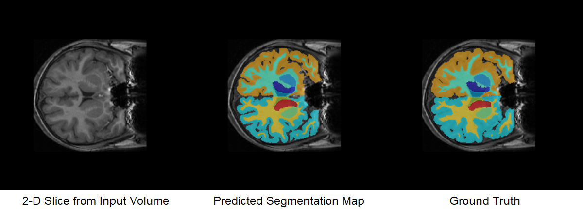
Predict the segmentation output for the preprocessed MRI volume. The predict (Deep Learning Toolbox) function supports gpuArray input, so it runs on the GPU. The segmentation output predictIm contains 32 channels corresponding to the segmentation label classes, such as "background", "leftCerebralCortex", and "rightThalamus". For each voxel, the predictIm function assigns a confidence score for every class. The confidence scores reflect the likelihood of the voxel being part of the corresponding class. This prediction is different from the final semantic segmentation output, which assigns each voxel to exactly one class.

predictIm = predict(net,volProc);

Test Time Augmentation

This example uses test time augmentation to improve segmentation accuracy by averaging out random errors in the individual network predictions.

By default, this example flips the MRI volume in the left-right direction, resulting in a flipped volume flippedData. The network output for the flipped volume is flipPredictIm. Set flipVal to false to skip the test time augmentation and speed up prediction.

flipVal = true;
if flipVal
    flippedData = fliplr(volProc);  
    flippedData = flip(flippedData,2);
    flippedData = flip(flippedData,1);
    flipPredictIm = predict(net,flippedData);
else
    flipPredictIm = [];  
end

Postprocess Segmentation Prediction

To get the final segmentation maps, postprocess the network output by using the postProcessBrainCANDIData helper function. The helper function is attached to this example as a supporting file. Because the postProcessBrainCANDIData function uses functions that are not supported on GPU, first transfer the data from GPU memory to host memory by using the gather function. The postProcessBrainCANDIData function performs these steps:

• Smoothing — Apply a 3-D Gaussian smoothing filter to reduce noise in the predicted segmentation masks.

• Morphological Filtering — Keep only the largest connected component of predicted segmentation masks to remove additional noise.

• Segmentation — Assign each voxel to the label class with the greatest confidence score for that voxel.

• Resizing — Resize the segmentation map to the original input volume size. Resizing the label image allows you to visualize the labels as an overlay on the grayscale MRI volume.

• Alignment — Rotate the segmentation map back to the orientation of the original input MRI volume.

The final segmentation result, predictedSegMaps, is a 3-D categorical array the same size as the original input volume. Each element corresponds to one voxel and has one categorical label.

predictIm = gather(predictIm);
flipPredictIm = gather(flipPredictIm);

predictedSegMaps = postProcessBrainCANDIData(predictIm,flipPredictIm,imSize, ...
    cropIdx,metaData,classNames,labelIDs);

Overlay a slice from the predicted segmentation map on a corresponding slice from the input volume using the labeloverlay function. Include all the brain structure labels except the background label. Because the labeloverlay function is not supported on GPU, transfer the test slice from GPU memory to host memory before calling labeloverlay.

sliceIdx = 80;
testSlice = rescale(vol(:,:,sliceIdx));
testSlice = gather(testSlice);
predSegMap = predictedSegMaps(:,:,sliceIdx);

B = labeloverlay(testSlice,predSegMap,IncludedLabels=2:32);
figure
montage({testSlice,B})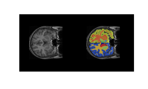

Quantify Segmentation Accuracy

Measure the segmentation accuracy by comparing the predicted segmentation labels with the ground truth labels drawn by clinical experts.

Create a pixelLabelDatastore (Computer Vision Toolbox) to store the labels. Because the NIfTI file format is a nonstandard image format, use the niftiread function to read the pixel label data.

pxds = pixelLabelDatastore(labelDirs,classNames,labelIDs,FileExtensions=".gz",...
    ReadFcn=@(X) uint8(niftiread(X)));

Read the ground truth labels from the pixel label datastore.

groundTruthLabel = read(pxds);
groundTruthLabel = groundTruthLabel{1};

Measure the segmentation accuracy using the dice function. This function computes the Dice index between the predicted and ground truth segmentations.

diceResult = zeros(length(classNames),1);
for j = 1:length(classNames)
    diceResult(j)= dice(groundTruthLabel==classNames(j),...
        predictedSegMaps==classNames(j));
end

Calculate the average Dice index across all labels for the MRI volume.

meanDiceScore = mean(diceResult);
disp("Average Dice score across all labels = " + meanDiceScore)

Average Dice score across all labels = 0.80789

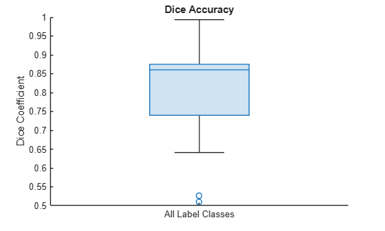
Visualize statistics about the Dice indices across all the label classes as a box chart. The middle blue line in the plot shows the median Dice index. The upper and lower bounds of the blue box indicate the 25th and 75th percentiles, respectively. Black whiskers extend to the most extreme data points that are not outliers.

figure
boxchart(diceResult)
title("Dice Accuracy")
xticklabels("All Label Classes")
ylabel("Dice Coefficient")

Compare Performance on CPU and GPU

Time the execution of the preprocessing and the segmentation steps on the GPU. To accurately time function execution on the GPU, use the gputimeit (Parallel Computing Toolbox) function, which runs a function multiple times to average out variation and compensate for overhead. The gputimeit function also ensures that all operations on the GPU are complete before recording the time.

volProc = gpuArray(volProc);
vol = gpuArray(vol);

timePreprocessGPU = gputimeit(@() preProcessBrainCANDIData(vol,metaData,cropSize,resample))

timePreprocessGPU = 
0.0077

timePredictGPU = gputimeit(@() predict(net,volProc))

timePredictGPU = 
0.2127

For comparison, time the same functions running on the CPU by using the timeit function.

volProc = gather(volProc);
vol = gather(vol);

timePreprocessCPU = timeit(@() preProcessBrainCANDIData(vol,metaData,cropSize,resample))

timePreprocessCPU = 
0.1235

timePredictCPU = timeit(@() predict(net,volProc))

timePredictCPU = 
8.1742

Compare the execution times.

figure
tiledlayout(1,2)

nexttile
bar([timePreprocessCPU,timePreprocessGPU])
grid on
ylabel("Execution Time (s)")
xticklabels(["CPU" "GPU"])
xlabel("Hardware")
title("Data Preprocessing")

nexttile
bar([timePredictCPU,timePredictGPU])
grid on
ylabel("Execution Time (s)")
xticklabels(["CPU" "GPU"])
xlabel("Hardware")
title("Segmentation")

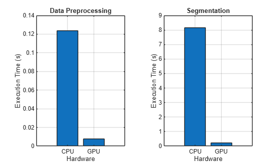
fprintf("Preprocessing speedup: %3.1fx \nPrediction speedup: %3.1fx", ...
timePreprocessCPU/timePreprocessGPU,timePredictCPU/timePredictGPU);

Preprocessing speedup: 16.1x 
Prediction speedup: 38.4x

These functions execute much faster on the GPU.

Running your code on a GPU is straightforward and can speed up your workflow. Generally, using a GPU is more beneficial when you are performing computations on large data sets, though the speedup you can achieve depends on your specific hardware and code.

References

[1] Billot, Benjamin, Douglas N. Greve, Oula Puonti, Axel Thielscher, Koen Van Leemput, Bruce Fischl, Adrian V. Dalca, and Juan Eugenio Iglesias. “SynthSeg: Domain Randomisation for Segmentation of Brain Scans of Any Contrast and Resolution.” ArXiv:2107.09559 [Cs, Eess], December 21, 2021. https://arxiv.org/abs/2107.09559.

[2] “NITRC: CANDI Share: Schizophrenia Bulletin 2008: Tool/Resource Info.” Accessed October 17, 2022. https://www.nitrc.org/projects/cs_schizbull08/.

[3] Frazier, J. A., S. M. Hodge, J. L. Breeze, A. J. Giuliano, J. E. Terry, C. M. Moore, D. N. Kennedy, et al. “Diagnostic and Sex Effects on Limbic Volumes in Early-Onset Bipolar Disorder and Schizophrenia.” Schizophrenia Bulletin 34, no. 1 (October 27, 2007): 37–46. https://doi.org/10.1093/schbul/sbm120.