Multilabel Diabetic Retinopathy Fundus Image Classification Using Deep Learning
This example shows how to classify diabetic retinopathy (DR) fundus images using a ResNet-101 deep neural network with transfer learning.
Diabetic retinopathy (DR) is a disease resulting from diabetes complications, causing non-reversible damage to retina blood vessels. This example shows how to classify DR fundus images into five stages: normal, mild, moderate, severe, and proliferative DR. In this example, you classify DR fundus images using a Resnet-101 based deep neural network trained to classify a DR fundus image into any of the five classes using transfer learning techniques.
Download Pretrained Network and Data Set
This example uses the Dataset for Diabetic Retinopathy (DDR) [1]. The DDR data set contains DR fundus images in the JPG file format and annotations in a .txt file. Run this code to download the data set and the pretrained network from the MathWorks® website and unzip the downloaded folder.
zipFile = matlab.internal.examples.downloadSupportFile("image","data/DRClassificationModelAndDataset.zip");
filepath = fileparts(zipFile);
unzip(zipFile,filepath)
The downloaded folder contains these files.
Preprocessed versions of the DR fundus images from the DDR data set.
Ground truth class labels in
.txtfiles.A sample image for visualization.
A pretrained deep neural network that you can use directly without training.
Load Pretrained Network
Load the pretrained network into the workspace.
trainedNetFile = fullfile(filepath,"trainedDRModel_resnet101.mat");
trainedNetData = load(trainedNetFile);
trainedNet = trainedNetData.trainedNet;
Observe the input size of the pretrained network.
inputSize = trainedNet.Layers(1).InputSize
inputSize = 1×3

   224   224     3
Perform Classification on Sample DR Fundus Image
Load the sample image from the downloaded data into the workspace.
sampleImgFile = fullfile(filepath,"sampleTrainImage.jpg");
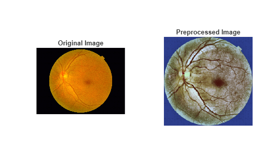
sampleImg = imread(sampleImgFile);Preprocess the sample image using the preprocessFundusImage helper function. The helper function is attached to this example as a supporting file.
sampleImgProc = preprocessFundusImage(sampleImg,inputSize(1:2));
Visualize the original and preprocessed sample image.
figure
tiledlayout(1,2)
nexttile
imshow(sampleImg)
title("Original Image")
nexttile
imshow(sampleImgProc)
title("Preprocessed Image")
Specify the five classes.
classNames = ["Normal","Mild DR","Moderate DR","Severe DR","Proliferate DR"];
numClasses = numel(classNames);
Predict the class of the sample image.
sampleScore = predict(trainedNet,sampleImgProc);
[~,sampleClassIdx] = max(sampleScore);
sampleClass = classNames(sampleClassIdx)
sampleClass =
"Proliferate DR"
Prepare Data for Training
Each of the DR fundus images in the data set have already been preprocessed using these steps.
Contrast Enhancement — The contrast of the L-channel of the image has been improved using contrast-limited adaptive histogram equalization (CLAHE) with a tile size of 8-by-8 and a clip limit of 0.05.
Noise Removal — Because contrast enhancement with the CLAHE method can introduce some noise, the image has been denoised using a Gaussian filter.
Cropping — The image has been cropped to eliminate the unnecessary black pixels around the retina.
Color Normalization — The images are from patients of varying ages and ethnic backgrounds, and have been captured under different lighting conditions. These factors affect the pixel intensity values of each image, causing unwanted variations. These variations have been normalized for each channel of the RGB image by subtracting the mean and then dividing by the standard deviation of the image.
Resize — The image has been resized to the input size of the deep neural network.
Read the train.txt file from the downloaded data set.
ddrTrainFile = fullfile(filepath,"train.txt");Create a table specifying the filename of the image to be used and the corresponding label by using the readTxtToDatatable helper function. The helper function is attached to this example as a supporting file. This example uses images with class labels 0 to 4. The class labels correspond to these classes.
0— Normal1— Mild DR2— Moderate DR3— Severe DR4— Proliferate DR
This example does not use images with class label 5, which indicates poor quality images.
ddrTrainTbl = readTxtToDatatable(ddrTrainFile);
The downloaded data set contains the training images in the folder processedDDRImagesTrain. Select the images specified in the table ddrTRainTbl, sort the data set by filename, and extract the labels for each image using the extractImgLabels helper function. The helper function is attached to this example as a supporting file.
imageDir = fullfile(filepath,"processedDDRImagesTrain");
[ddrTrainImages,ddrTrainLabels] = extractImgLabels(ddrTrainTbl,imageDir);
Visualize the class distribution in the training data set. Observe the class imbalance in the training data.
ddrTrainLabelDist = tabulate(ddrTrainLabels);
ddrTrainLabelDist = array2table(ddrTrainLabelDist,VariableNames=["Labels","GroupCount","Percent"])
ddrTrainLabelDist=5×3 table
    Labels    GroupCount    Percent
    ______    __________    _______

      0          3015       46.557
      1           485       7.4892
      2          2114       32.644
      3           184       2.8413
      4           678       10.469
Create Training Datastore
Create a datastore for the training data using the createFundusImageDatastore helper function. The helper function is attached to this example as a supporting file. The function performs these operations.
Hot encodes the labels.
Augments the training data to reduce class imbalance by specifying
doAugmentationastrue.Sets the specified minibatch size while creating the datastore.
miniBatchSizeTrain = 32;
doAugmentation = true;
[dataTrain,encodedLabelsTrain] = createFundusImageDatastore(ddrTrainImages,ddrTrainLabels,numClasses,inputSize,doAugmentation,miniBatchSizeTrain);
Visualize the number of labels for each class in the training datastore using a bar chart.
numSamplesPerClass = sum(encodedLabelsTrain,1);
figure
bar(numSamplesPerClass)
ylabel("Number of Samples")
xticklabels(classNames)
Create Validation and Test Datastore
Read the valid.txt file from the downloaded data set to read the test data. Create a test datastore similar to the training datastore. Do not perform augmentation on the test data set.
ddrTestFile = fullfile(filepath,"valid.txt");
ddrTestTbl = readTxtToDatatable(ddrTestFile);
imageDir = fullfile(filepath,"processedDDRImagesTest");
[ddrTestImages,ddrTestLabels] = extractImgLabels(ddrTestTbl,imageDir);
miniBatchSizeTest = 16;
doAugmentation = false;
[dataTest,encodedLabelsTest] = createFundusImageDatastore(ddrTestImages,ddrTestLabels,numClasses,inputSize,doAugmentation,miniBatchSizeTest);
Define Network Architecture
Load a pretrained ResNet-101 network using the imagePretrainedNetwork (Deep Learning Toolbox) function. Using the ResNet-101 pretrained network requires the Deep Learning Toolbox Model for ResNet-101 Network™ support package. If the support package is not installed, then the function provides a download link.
net = imagePretrainedNetwork("resnet101",NumClasses=numClasses);Specify Training Options
Specify the training options using the trainingOptions (Deep Learning Toolbox) function. Train the object detector using the SGDM solver for a maximum of 15 epochs.
options = trainingOptions("sgdm", ...
    InitialLearnRate=5e-4, ...
    LearnRateDropFactor=0.2, ...
    LearnRateDropPeriod=5, ...
    LearnRateSchedule="cosine", ...
    MiniBatchSize=32, ...
    MaxEpochs=15, ...
    Verbose= false, ...
    ValidationData=dataTest, ...
    ValidationFrequency=10, ...
    Metrics="rmse", ...
    Plots="training-progress");
Train Network
To train the detector, set the doTraining variable to true. Train the detector by using the trainnet (Deep Learning Toolbox) function. Use focal cross entropy as the loss function to handle class imbalance by dynamically scaling the loss of each sample based on its difficulty. The trainnet function utilizes a GPU if available. Using a GPU for training requires a Parallel Computing Toolbox™ license and a compatible GPU device. For details on supported devices, refer to the GPU Computing Requirements (Parallel Computing Toolbox). If a GPU is not available, the trainnet function uses the CPU. You can specify the execution environment by using the ExecutionEnvironment training option.
doTraining = false;
lossFcn = @(Y,T)focalCrossEntropy(Y,T,ClassificationMode="single-label");
if doTraining
    trainedNet = trainnet(dataTrain,net,lossFcn,options);
    saveTrainedNetFile = fullfile(filepath,"trainedDRModel_resnet101.mat");
    save(saveTrainedNetFile,"trainedNet")
else
    trainedNetFile = fullfile(filepath,"trainedDRModel_resnet101.mat");
    trainedNetData = load(trainedNetFile);
    trainedNet = trainedNetData.trainedNet;
end
Evaluate Network Using Test Data
Predict the classes for the test data using the trained network.
predScores = minibatchpredict(trainedNet,dataTest);
Extract the ground truth labels for the test data.
[~,trueClassIndices] = max(encodedLabelsTest,[],2);
trueLabels = classNames(trueClassIndices)';
Create an rocmetrics (Deep Learning Toolbox) object for the predicted scores for region of convergence (ROC) evaluation. Include additional metrics, such as positive predictive value (PPV), F1 score, and accuracy, in the ROC evaluation.
rocObj = rocmetrics(trueLabels,predScores,classNames,AdditionalMetrics=["ppv","f1score","accu"]);
metricsTbl = rocObj.Metrics;
aucScores = auc(rocObj);
Create subtables for each class for evaluation.
subtables = containers.Map;
for i = 1:length(classNames)
    className = classNames{i};
    rowIdx = strcmp(metricsTbl.ClassName,className);
    subtables(className) = metricsTbl(rowIdx,:);
end
Plot F1 Scores
Visualize the plot of F1 score against threshold for each class.
tiledlayout(2,3)
for i = 1:length(classNames)
    className = classNames{i};
    nexttile
    plot(subtables(className).Threshold,subtables(className).F1Score);
    xlabel("Threshold")
    ylabel("F1 Score")
    title(className)
end

Compute Classification Metrics
Compute metrics such as PPV, F1 score, accuracy, and area under the ROC curve (AUC) for each class.
results = table(Size=[length(classNames) 5], ...
                VariableTypes=["string","double","double","double","double"], ...
                VariableNames=["ClassName","PPV","F1Score","Accuracy","AUC"]);

for i = 1:length(classNames)
    className = classNames{i};
    [maxF1Score,threshIdx] = max(subtables(className).F1Score);
    maxAcc = subtables(className).Accuracy(threshIdx);
    maxPPV = subtables(className).PositivePredictiveValue(threshIdx);
    results.ClassName(i) = className;
    results.PPV(i) = maxPPV;
    results.F1Score(i) = maxF1Score;
    results.Accuracy(i) = maxAcc;
    results.AUC(i) = aucScores(i);
end
disp(results)
ClassName PPV F1Score Accuracy AUC
________________ ________ _______ ________ _______
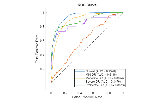
"Normal" 0.82884 0.88745 0.86655 0.93284
"Mild DR" 0.070423 0.12647 0.56402 0.61163
"Moderate DR" 0.65297 0.73616 0.81515 0.88939
"Severe DR" 0.40741 0.44444 0.9752 0.84756
"Proliferate DR" 0.56667 0.6 0.93868 0.88733
Plot ROC curve
Plot the ROC curve for the predictions on the test data set.
figure
plot(rocObj,ShowModelOperatingPoint=false)
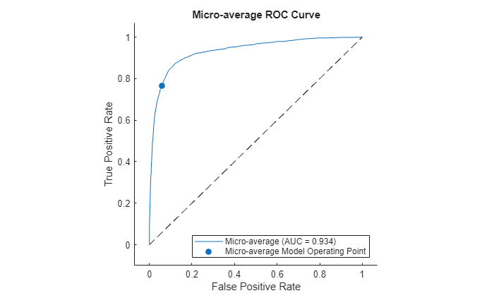
Plot the micro-average ROC curve.
figure
plot(rocObj,AverageCurveType="micro",ClassNames=[])
title("Micro-average ROC Curve")
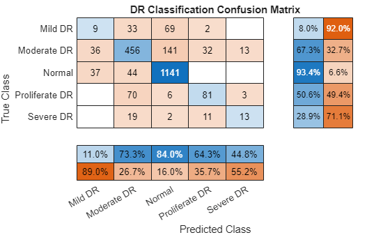
Visualize Confusion Chart
Visualize a multiclass confusion chart for the predictions.
[~,predClassIndices] = max(predScores,[],2);
predLabels = classNames(predClassIndices)';
figure
confusionchart(trueLabels,predLabels,RowSummary="row-normalized",ColumnSummary="column-normalized",Title="DR Classification Confusion Matrix")
Explainability
The model estimates the probability of each class being present in the input image. The predicted class is the class with the maximum probability. Investigate the network predictions on two test images. GradCAM is an explainability technique that uses the gradient of class scores relative to the convolutional features of the network. It helps to identify which regions of the image contribute to each class label. Use GradCAM to see which parts of the image the network considers significant for each of the true classes.
testImageIdx = [50 115];
Predict the scores and class for the first test image.
testImg1 = imread(ddrTestImages(testImageIdx(1)));
testImg1 = imresize(testImg1,inputSize(1:2));
scoresTestImg1 = predict(trainedNet,single(testImg1))';
[~,predClassIdx1] = max(scoresTestImg1);
predLabel1 =  classNames(predClassIdx1)
predLabel1 =
"Mild DR"
trueClassIdx1 = logical(encodedLabelsTest(testImageIdx(1),:)');
trueLabel1 = classNames(trueClassIdx1)
trueLabel1 =
"Mild DR"
Generate the GradCAM map for each class label for the first test image.
map1 = gradCAM(trainedNet,testImg1,1:numClasses);
Visualize the scores and the GradCAM map for each class for the first test image.
tbl1 = table(classNames',scoresTestImg1,VariableNames=["Class","Score"]);
disp(tbl1)
         Class            Score
    ________________    _________

    "Normal"              0.22795
    "Mild DR"             0.61959
    "Moderate DR"         0.14735
    "Severe DR"         0.0016136
    "Proliferate DR"    0.0034912
figure
tiledlayout("flow")
nexttile
imshow(testImg1)
title("Test Image 1")
for i = 1:numClasses
    nexttile
    imshow(testImg1)
    hold on
    title(classNames(i))
    imagesc(map1(:,:,i),AlphaData=0.5)
    hold off
end
colormap jet

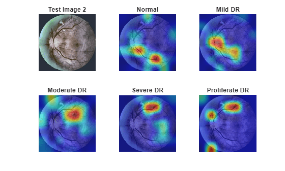
Predict the scores and class for the second test image.
testImg2 = imread(ddrTestImages(testImageIdx(2)));
testImg2 = imresize(testImg2,inputSize(1:2));
scoresTestImg2 = predict(trainedNet,single(testImg2))';
[~,predClassIdx2] = max(scoresTestImg2);
predLabel2 =  classNames(predClassIdx2)
predLabel2 =
"Moderate DR"
trueClassIdx2 = logical(encodedLabelsTest(testImageIdx(2),:)');
trueLabel2 = classNames(trueClassIdx2)
trueLabel2 =
"Moderate DR"
Generate the GradCAM map for each class label for the second test image.
map2 = gradCAM(trainedNet,testImg2,1:numClasses);
Visualize the scores and the GradCAM map for each class for the second test image.
tbl2 = table(classNames',scoresTestImg2,VariableNames=["Class","Score"]);
disp(tbl2)
         Class           Score
    ________________    ________

    "Normal"             0.15063
    "Mild DR"            0.17122
    "Moderate DR"         0.5742
    "Severe DR"         0.074886
    "Proliferate DR"    0.029068
figure
tiledlayout("flow")
nexttile
imshow(testImg2)
title("Test Image 2")
for i = 1:numClasses
    nexttile
    imshow(testImg2)
    hold on
    title(classNames(i))
    imagesc(map2(:,:,i),AlphaData=0.5)
    hold off
end
colormap jet
References
[1] A General-purpose High-quality Dataset for Diabetic Retinopathy Classification, Lesion Segmentation and Lesion Detection. GitHub. https://github.com/nkicsl/DDR-dataset.
[2] Alyoubi, Wejdan L., Maysoon F. Abulkhair, and Wafaa M. Shalash. "Diabetic Retinopathy Fundus Image Classification and Lesions Localization System Using Deep Learning." Sensors 21, no. 11 (May 26, 2021): 3704. https://doi.org/10.3390/s21113704.
[3] Li, Tao, Yingqi Gao, Kai Wang, Song Guo, Hanruo Liu, and Hong Kang. "Diagnostic Assessment of Deep Learning Algorithms for Diabetic Retinopathy Screening." Information Sciences 501 (October 2019): 511–22. https://doi.org/10.1016/j.ins.2019.06.011.
See Also
imagePretrainedNetwork (Deep Learning Toolbox) | trainingOptions (Deep Learning Toolbox) | trainnet (Deep Learning Toolbox)