MPC Prediction Models

Model predictive controllers use plant, disturbance, and noise models for prediction and state estimation. The different signal types are described in MPC Signal Types. The model structure used in an MPC controller appears in the following illustration.

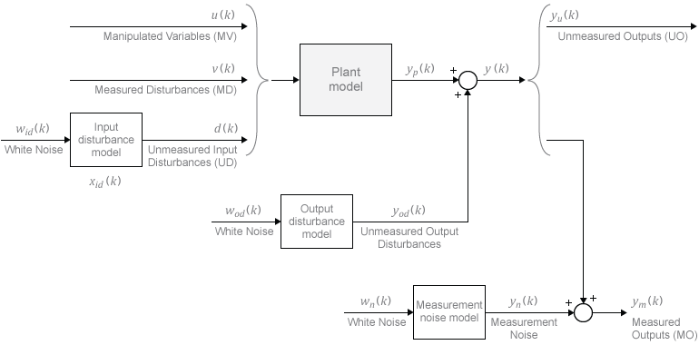
Plant Model

You can specify the plant model in one of the following linear-time-invariant (LTI) formats:

• Numeric LTI models — Transfer function (tf), state space (ss), zero-pole-gain (zpk)

• Identified models (requires System Identification Toolbox™) — idss (System Identification Toolbox), idtf (System Identification Toolbox), idproc (System Identification Toolbox), and idpoly (System Identification Toolbox)

The MPC controller performs all estimation and optimization calculations using a discrete-time, delay-free, state-space system with dimensionless input and output variables. Therefore, when you specify a plant model in the MPC controller, the software performs the following, if needed:

1. Conversion to state space — The ss command converts the supplied model to an LTI state-space model.

2. Discretization or resampling — If the model sample time differs from the MPC controller sample time (defined in the Ts property), one of the following occurs:

   • If the model is continuous time, the c2d command converts it to a discrete-time LTI object using the controller sample time.

   • If the model is discrete time, the d2d command resamples it to generate a discrete-time LTI object using the controller sample time.

3. Delay removal — If the discrete-time model includes any input, output, or internal delays, the absorbDelay command replaces them with the appropriate number of poles at z = 0, increasing the total number of discrete states. The InputDelay, OutputDelay, and InternalDelay properties of the resulting state-space model are all zero.

4. Conversion to dimensionless input and output variables — The MPC controller enables you to specify a scale factor for each plant input and output variable. If you do not specify scale factors, they default to 1. The software converts the plant input and output variables to dimensionless form as follows:

   $\begin{array}{c}{x}_p\left(k+1\right)=A_p{x}_p\left(k\right)+B{S}_i{u}_p\left(k\right)\\ y_p\left(k\right)=S_o^{-1}C{x}_p\left(k\right)+S_o^{-1}D{S}_i{u}_p\left(k\right).\end{array}$

   where A_p, B, C, and D are the constant zero-delay state-space matrices from step 3, and:

   • S_i is a diagonal matrix of input scale factors in engineering units.

   • S_o is a diagonal matrix of output scale factors in engineering units.

   • x_p is the state vector from step 3 in engineering units (including any absorbed delay states). No scaling is performed on state variables.

   • u_p is a vector of dimensionless plant input variables, including manipulated variables, measured disturbances, and unmeasured input disturbances.

   • y_p is a vector of dimensionless plant output variables.

   The resulting plant model has the following equivalent form:

   $\begin{array}{c}{x}_p\left(k+1\right)=A_p{x}_p\left(k\right)+B_{pu}u\left(k\right)+B_{pv}v\left(k\right)+B_{pd}d\left(k\right)\\ y_p\left(k\right)=C_p{x}_p\left(k\right)+D_{pu}u\left(k\right)+D_{pv}v\left(k\right)+D_{pd}d\left(k\right).\end{array}$

   Here, $C_p=S_o^{-1}C$, B_pu, B_pv, and B_pd are the corresponding columns of BS_i. Also, D_pu, D_pv, and D_pd are the corresponding columns of $S_o^{-1}D{S}_i$. Finally, u(k), v(k), and d(k) are the dimensionless manipulated variables, measured disturbances, and unmeasured input disturbances, respectively.

   The MPC controller enforces the restriction of D_pu = 0, which means that the controller does not allow direct feedthrough from any manipulated variable to any plant output.

Input Disturbance Model

If your plant model includes unmeasured input disturbances, d(k), the input disturbance model specifies the signal type and characteristics of d(k). See Controller State Estimation for more information about the model.

The getindist command provides access to the model in use.

The input disturbance model is a key factor that influences the following controller performance attributes:

• Dynamic response to apparent disturbances — The character of the controller response when the measured plant output deviates from its predicted trajectory, due to an unknown disturbance or modeling error.

• Asymptotic rejection of sustained disturbances — If the disturbance model predicts a sustained disturbance, controller adjustments continue until the plant output returns to its desired trajectory, emulating a classical integral feedback controller.

You can provide the input disturbance model as an LTI state-space (ss), transfer function (tf), or zero-pole-gain (zpk) object using setindist. The MPC controller converts the input disturbance model to a discrete-time, delay-free, LTI state-space system using the same steps used to convert the plant model. The result is:

$\begin{array}{c}{x}_{id}\left(k+1\right)=A_{id}{x}_{id}\left(k\right)+B_{id}{w}_{id}\left(k\right)\\ d\left(k\right)=C_{id}{x}_{id}\left(k\right)+D_{id}{w}_{id}\left(k\right).\end{array}$

where A_id, B_id, C_id, and D_id are constant state-space matrices, and:

• x_id(k) is a vector of n_xid ≥ 0 input disturbance model states.

• d_k(k) is a vector of n_d dimensionless unmeasured input disturbances.

• w_id(k) is a vector of n_id ≥ 1 dimensionless white noise inputs, assumed to have zero mean and unit variance.

If you do not provide an input disturbance model, then the controller uses a default model, which has integrators with dimensionless unity gain added to its outputs. An integrator is added for each unmeasured input disturbance, unless doing so would cause a violation of state observability. In this case, a static system with dimensionless unity gain is used instead.

Output Disturbance Model

The output disturbance model is a special case of the more general input disturbance model. Its output, y_od(k), is directly added to the plant output rather than affecting the plant states. The output disturbance model specifies the signal type and characteristics of y_od(k), and it is often used in practice. See Controller State Estimation for more details about the model.

The getoutdist command provides access to the output disturbance model in use.

You can specify a custom output disturbance model as an LTI state-space (ss), transfer function (tf), or zero-pole-gain (zpk) object using setoutdist. Using the same steps as for the plant model, the MPC controller converts the specified output disturbance model to a discrete-time, delay-free, LTI state-space system. The result is:

$\begin{array}{c}{x}_{od}\left(k+1\right)=A_{od}{x}_{od}\left(k\right)+B_{od}{w}_{od}\left(k\right)\\ y_{od}\left(k\right)=C_{od}{x}_{od}\left(k\right)+D_{od}{w}_{od}\left(k\right).\end{array}$

where A_od, B_od, C_od, and D_od are constant state-space matrices, and:

• x_od(k) is a vector of n_xod ≥ 1 output disturbance model states.

• y_od(k) is a vector of n_y dimensionless output disturbances to be added to the dimensionless plant outputs.

• w_od(k) is a vector of n_od dimensionless white noise inputs, assumed to have zero mean and unit variance.

If you do not specify an output disturbance model, then the controller uses a default model, which has integrators with dimensionless unity gain added to some or all of its outputs. These integrators are added according to the following rules:

• No disturbances are estimated, that is no integrators are added, for unmeasured plant outputs.

• An integrator is added for each measured output in order of decreasing output weight.

  • For time-varying weights, the sum of the absolute values over time is considered for each output channel.

  • For equal output weights, the order within the output vector is followed.

• For each measured output, an integrator is not added if doing so would cause a violation of state observability. Instead, a gain with a value of zero is used instead.

If there is an input disturbance model, then the controller adds any default integrators to that model before constructing the default output disturbance model.

Measurement Noise Model

One controller design objective is to distinguish disturbances, which require a response, from measurement noise, which should be ignored. The measurement noise model specifies the expected noise type and characteristics. See Controller State Estimation for more details about the model.

Using the same steps as for the plant model, the MPC controller converts the measurement noise model to a discrete-time, delay-free, LTI state-space system. The result is:

$\begin{array}{c}{x}_n\left(k+1\right)=A_n{x}_n\left(k\right)+B_n{w}_n\left(k\right)\\ y_n\left(k\right)=C_n{x}_n\left(k\right)+D_n{w}_n\left(k\right).\end{array}$

Here, A_n, B_n, C_n, and D_n are constant state space matrices, and:

• x_n(k) is a vector of n_xn ≥ 0 noise model states.

• y_n(k) is a vector of n_ym dimensionless noise signals to be added to the dimensionless measured plant outputs.

• w_n(k) is a vector of n_n ≥ 1 dimensionless white noise inputs, assumed to have zero mean and unit variance.

If you do not supply a noise model, the default is a unity static gain: n_xn = 0, D_n is an n_ym-by-n_ym identity matrix, and A_n, B_n, and C_n are empty.

For an mpc controller object, mpcobj, the property mpcobj.Model.Noise provides access to the measurement noise model.

Note

If the minimum eigenvalue of $$D_n{D}_n^T$$ is less than 1x10^–8, the MPC controller adds 1x10^–4 to each diagonal element of D_n. This adjustment makes a successful default Kalman gain calculation more likely.