Adaptive Cruise Control with Sensor Fusion
This example shows how to implement a sensor fusion-based automotive adaptive cruise controller for a vehicle traveling on a curved road using sensor fusion.
In this example, you:
Review a control system that combines sensor fusion and an adaptive cruise controller (ACC). Two variants of ACC are provided: a classical controller and an Adaptive Cruise Control System block from Model Predictive Control Toolbox.
Test the control system in a closed-loop Simulink model using synthetic data generated by the Automated Driving Toolbox.
Configure the code generation settings for software-in-the-loop simulation, and automatically generate code for the control algorithm.
Introduction
An adaptive cruise control system is a control system that modifies the speed of the ego vehicle in response to conditions on the road. As in regular cruise control, the driver sets a desired speed for the car; in addition, the adaptive cruise control system can slow the ego vehicle down if there is another vehicle moving slower in the lane in front of it.
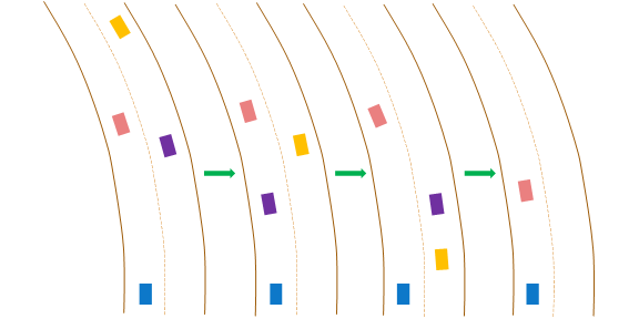
For the ACC to work correctly, the ego vehicle must determine how the lane in front of it curves, and which car is the 'lead car', that is, in front of the ego vehicle in the lane. A typical scenario from the viewpoint of the ego vehicle is shown in the following figure. The ego vehicle (blue) travels along a curved road. At the beginning, the lead car is the pink car. Then the purple car cuts into the lane of the ego vehicle and becomes the lead car. After a while, the purple car changes to another lane, and the pink car becomes the lead car again. The pink car remains the lead car afterward. The ACC design must react to the change in the lead car on the road.
Current ACC designs rely mostly on range and range rate measurements obtained from radar, and are designed to work best along straight roads. An example of such a system is given in Adaptive Cruise Control System Using Model Predictive Control (Model Predictive Control Toolbox) and in Automotive Adaptive Cruise Control Using FMCW Technology (Radar Toolbox). Moving from advanced driver-assistance system (ADAS) designs to more autonomous systems, the ACC must address the following challenges:
Estimating the relative positions and velocities of the cars that are near the ego vehicle and that have significant lateral motion relative to the ego vehicle.
Estimating the lane ahead of the ego vehicle to find which car in front of the ego vehicle is the closest one in the same lane.
Reacting to aggressive maneuvers by other vehicles in the environment, in particular, when another vehicle cuts into the ego vehicle lane.
This example demonstrates two main additions to existing ACC designs that meet these challenges: adding a sensor fusion system and updating the controller design based on model predictive control (MPC). A sensor fusion and tracking system that uses both vision and radar sensors provides the following benefits:
It combines the better lateral measurement of position and velocity obtained from vision sensors with the range and range rate measurement from radar sensors.
A vision sensor can detect lanes, provide an estimate of the lateral position of the lane relative to the ego vehicle, and position the other cars in the scene relative to the ego vehicle lane. This example assumes ideal lane detection.
An advanced MPC controller adds the ability to react to more aggressive maneuvers by other vehicles in the environment. In contrast to a classical controller that uses a PID design with constant gains, the MPC controller regulates the velocity of the ego vehicle while maintaining a strict safe distance constraint. Therefore, the controller can apply more aggressive maneuvers when the environment changes quickly in a similar way to what a human driver would do.
Overview of Test Bench Model and Simulation Results
Get a list of systems that are open now so any systems opened during this example can be closed at the end, then open the main Simulink model.
startingOpenSystems = find_system('MatchFilter', @Simulink.match.allVariants);
open_system('ACCTestBenchExample')
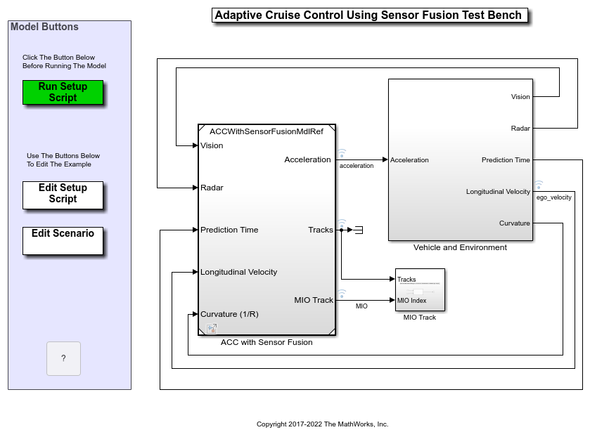
The model contains two main subsystems:
ACC with Sensor Fusion, which models the sensor fusion and controls the longitudinal acceleration of the vehicle. This component allows you to select either a classical or model predictive control version of the design.
A Vehicle and Environment subsystem, which models the motion of the ego vehicle and models the environment. A simulation of radar and vision sensors provides synthetic data to the control subsystem.
To run the associated initialization script before running the model, in the Simulink model, click Run Setup Script or, at the command prompt, type the following:
helperACCSetUp
The script loads certain constants needed by the Simulink model, such as the scenario object, vehicle parameters, and ACC design parameters. The default ACC is the classical controller. The script also creates buses that are required for defining the inputs into and outputs for the control system referenced model. These buses must be defined in the workspace before model compilation. When the model compiles, additional Simulink buses are automatically generated by their respective blocks.
To plot the results of the simulation and depict the surroundings of the ego vehicle, including the tracked objects, use the Bird's-Eye Scope. The Bird's-Eye Scope is a model-level visualization tool that you can open from the Simulink toolstrip. On the Simulation tab, under Review Results, click Bird's-Eye Scope. After opening the scope, click Find Signals to set up the signals. The following commands run the simulation to 15 seconds to get a mid-simulation picture and run again all the way to end of the simulation to gather results.
sim('ACCTestBenchExample','StopTime','15') %Simulate 15 seconds
sim('ACCTestBenchExample') %Simulate to end of scenario
ans =

  Simulink.SimulationOutput:
                logsout: [1x1 Simulink.SimulationData.Dataset]
                   tout: [151x1 double]

     SimulationMetadata: [1x1 Simulink.SimulationMetadata]
           ErrorMessage: [0x0 char]
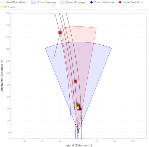

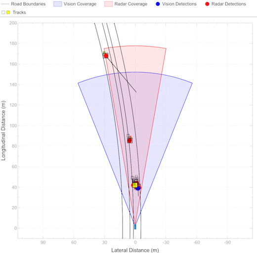
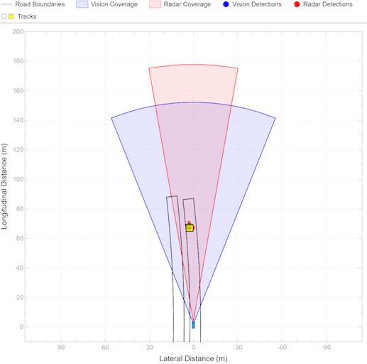
The Bird's-Eye Scope shows the results of the sensor fusion. It shows how the radar and vision sensors detect the vehicles within their sensors coverage areas. It also shows the tracks maintained by the Multi-Object Tracker block. The yellow track shows the most important object (MIO): the closest track in front of the ego vehicle in its lane. We see that at the beginning of the scenario, the most important object is the fast-moving car ahead of the ego vehicle. When the passing car gets closer to the slow-moving car, it crosses to the left lane, and the sensor fusion system recognizes it to be the MIO. This car is much closer to the ego vehicle and much slower than it. Thus, the ACC must slow the ego vehicle.
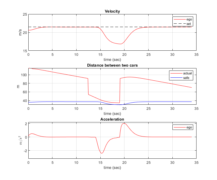
In the following results for the classical ACC system, the:
Top plot shows the ego vehicle velocity.
Middle plot shows the relative distance between the ego vehicle and lead car.
Bottom plot shows the ego vehicle acceleration.
In this example, the raw data from the Tracking and Sensor Fusion system is used for ACC design without post-processing. You can expect to see some 'spikes' (middle plot) due to the uncertainties in the sensor model especially when another car cuts into or leaves the ego vehicle lane.
To view the simulation results, use the following command.
helperPlotACCResults(logsout,default_spacing,time_gap)
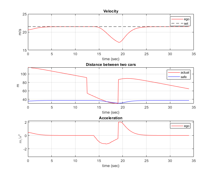
In the first 11 seconds, the lead car is far ahead of the ego vehicle (middle plot). The ego vehicle accelerates and reaches the velocity set by the driver (top plot).
Another car becomes the lead car from 11 to 20 seconds when the car cuts into the ego vehicle lane (middle plot). When the distance between the lead car and the ego vehicle is large (11-15 seconds), the ego vehicle still travels at the driver-set velocity. When the distance becomes small (15-20 seconds), the ego vehicle decelerates to maintain a safe distance from the lead car (top plot).
From 20 to 34 seconds, the car in front moves to another lane, and a new lead car appears (middle plot). Because the distance between the lead car and the ego vehicle is large, the ego vehicle accelerates until it reaches the driver-set velocity at 27 seconds. Then, the ego vehicle continues to travel at the driver-set velocity (top plot).
The bottom plot demonstrates that the acceleration is within the range [-3,2] m/s^2. The smooth transient behavior indicates that the driver comfort is satisfactory.
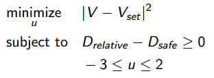
In the MPC-based ACC design, the underlying optimization problem is formulated by tracking the driver-set velocity subject to enforcing a safe distance from the lead car. The MPC controller design is described in the Adaptive Cruise Controller section. To run the model with the MPC design, first activate the MPC variant, and then run the following commands. This step requires Model Predictive Control Toolbox software. You can check the existence of this license using the following code. If no code exists, a sample of similar results is depicted.
hasMPCLicense = license('checkout','MPC_Toolbox');
if hasMPCLicense
    controller_type = 2;
    sim('ACCTestBenchExample','StopTime','15') %Simulate 15 seconds
    sim('ACCTestBenchExample') %Simulate to end of scenario
else
    load data_mpc
end
-->Converting model to discrete time.
-->Assuming output disturbance added to measured output #2 is integrated white noise.
   Assuming no disturbance added to measured output #1.
-->"Model.Noise" is empty. Assuming white noise on each measured output.

ans =

  Simulink.SimulationOutput:
                logsout: [1x1 Simulink.SimulationData.Dataset]
                   tout: [151x1 double]

     SimulationMetadata: [1x1 Simulink.SimulationMetadata]
           ErrorMessage: [0x0 char]

-->Converting model to discrete time.
-->Assuming output disturbance added to measured output #2 is integrated white noise.
   Assuming no disturbance added to measured output #1.
-->"Model.Noise" is empty. Assuming white noise on each measured output.
In the simulation results for the MPC-based ACC, similar to the classical ACC design, the objectives of speed and spacing control are achieved. Compared to the classical ACC design, the MPC-based ACC is more aggressive as it uses full throttle or braking for acceleration or deceleration. This behavior is due to the explicit constraint on the relative distance. The aggressive behavior may be preferred when sudden changes on the road occur, such as when the lead car changes to be a slow car. To make the controller less aggressive, open the mask of the Adaptive Cruise Control System block, and reduce the value of the Controller Behavior parameter. As previously noted, the spikes in the middle plot are due to the uncertainties in the sensor model.
To view the results of the simulation with the MPC-based ACC, use the following command.
helperPlotACCResults(logsout,default_spacing,time_gap)
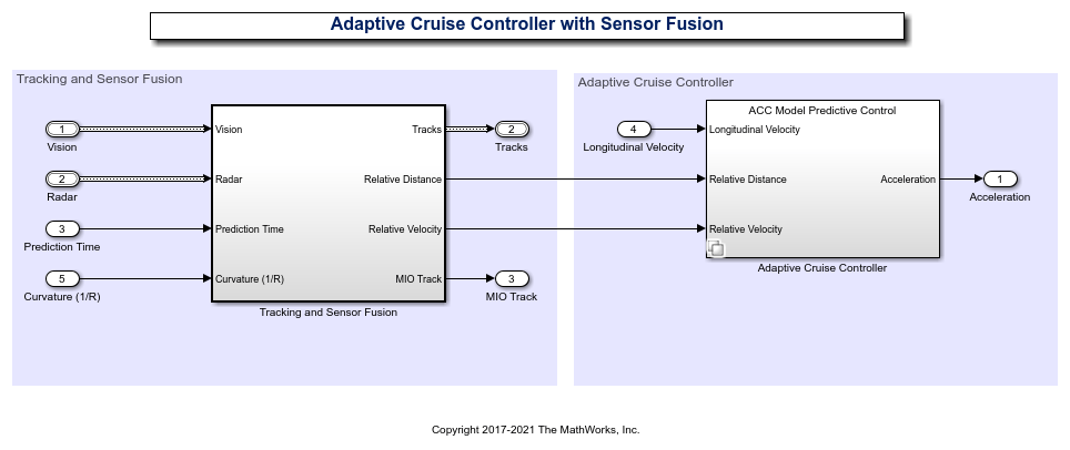
In the following, the functions of each subsystem in the Test Bench Model are described in more detail. The Adaptive Cruise Controller with Sensor Fusion subsystem contains two main components:
Tracking and Sensor Fusion subsystem
Adaptive Cruise Controller subsystem
open_system('ACCTestBenchExample/ACC with Sensor Fusion')
Tracking and Sensor Fusion
The Tracking and Sensor Fusion subsystem processes vision and radar detections coming from the Vehicle and Environment subsystem and generates a comprehensive situation picture of the environment around the ego vehicle. Also, it provides the ACC with an estimate of the closest car in the lane in front of the ego vehicle.
open_system('ACCWithSensorFusionMdlRef/Tracking and Sensor Fusion')
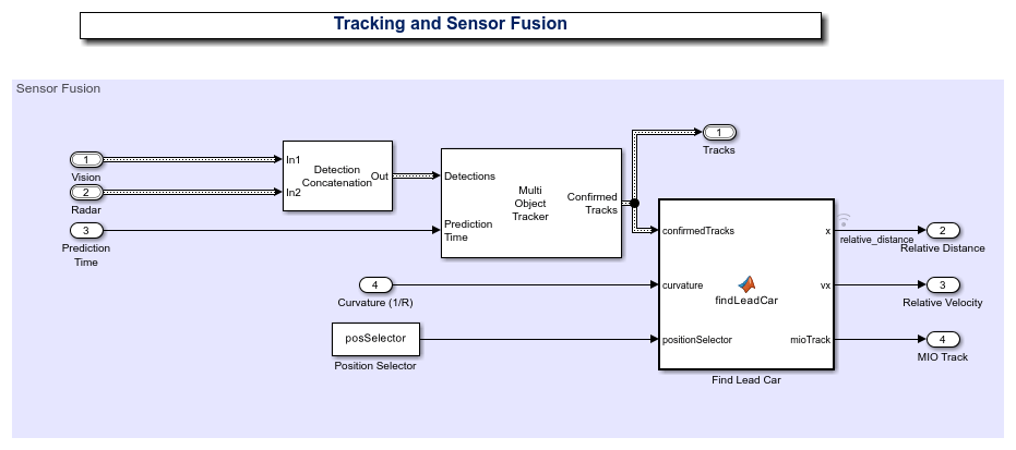
The main block of the Tracking and Sensor Fusion subsystem is the Multi-Object Tracker block, whose inputs are the combined list of all the sensor detections and the prediction time. The output from the Multi-Object Tracker block is a list of confirmed tracks.
The Detection Concatenation block concatenates the vision and radar detections. The prediction time is driven by a clock in the Vehicle and Environment subsystem.
The Detection Clustering block clusters multiple radar detections, since the tracker expects at most one detection per object per sensor.
The findLeadCar MATLAB function block finds which car is closest to the ego vehicle and ahead of it in same the lane using the list of confirmed tracks and the curvature of the road. This car is referred to as the lead car, and may change when cars move into and out of the lane in front of the ego vehicle. The function provides the position and velocity of the lead car relative to the ego vehicle and an index to the most important object (MIO) track.
Adaptive Cruise Controller
The adaptive cruise controller has two variants: a classical design (default) and an MPC-based design. For both designs, the following design principles are applied. An ACC equipped vehicle (ego vehicle) uses sensor fusion to estimate the relative distance and relative velocity to the lead car. The ACC makes the ego vehicle travel at a driver-set velocity while maintaining a safe distance from the lead car. The safe distance between lead car and ego vehicle is defined as

where the default spacing  , and time gap
  are design parameters and
  is the longitudinal velocity of the ego vehicle. The ACC generates the longitudinal acceleration for the ego vehicle based on the following inputs:
Longitudinal velocity of ego vehicle
Relative distance between lead car and ego vehicle (from the Tracking and Sensor Fusion system)
Relative velocity between lead car and ego vehicle (from the Tracking and Sensor Fusion system)
Considering the physical limitations of the ego vehicle, the longitudinal acceleration is constrained to the range [-3,2]  .
.
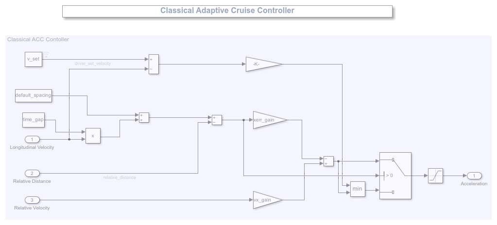
In the classical ACC design, if the relative distance is less than the safe distance, then the primary goal is to slow down and maintain a safe distance. If the relative distance is greater than the safe distance, then the primary goal is to reach driver-set velocity while maintaining a safe distance. These design principles are achieved through the Min and Switch blocks.
open_system('ACCWithSensorFusionMdlRef/Adaptive Cruise Controller/ACC Classical')
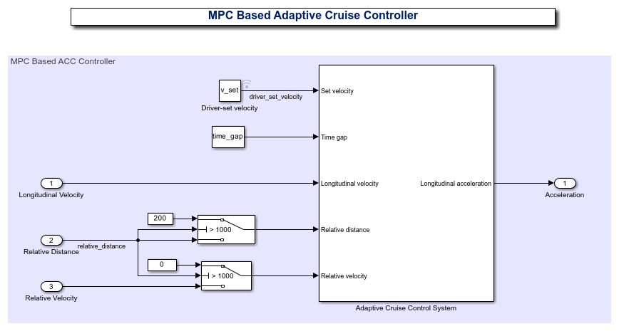
In the MPC-based ACC design, the underlying optimization problem is formulated by tracking the driver-set velocity subject to a constraint. The constraint enforces that relative distance is always greater than the safe distance.
To configure the Adaptive Cruise Control System block, use the parameters defined in the helperACCSetUp file. For example, the linear model for ACC design  , and is obtained from vehicle dynamics. The two Switch blocks implement simple logic to handle large numbers from the sensor (for example, the sensor may return
 Inf when it does not detect an MIO).
open_system('ACCWithSensorFusionMdlRef/Adaptive Cruise Controller/ACC Model Predictive Control')
For more information on MPC design for ACC, see Adaptive Cruise Control System Using Model Predictive Control (Model Predictive Control Toolbox).
Vehicle and Environment
The Vehicle and Environment subsystem is composed of two parts:
Vehicle Dynamics and Global Coordinates
Actor and Sensor Simulation
open_system('ACCTestBenchExample/Vehicle and Environment')
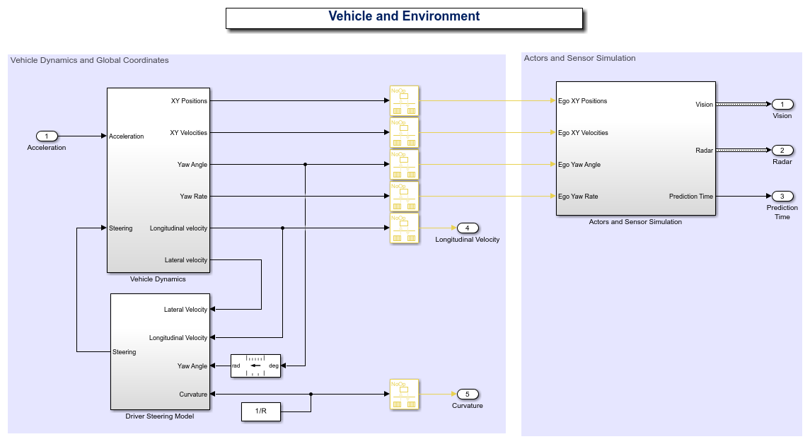
The Vehicle Dynamics subsystem models the vehicle dynamics with the Bicycle Model - Force Input block from the Automated Driving Toolbox. The vehicle dynamics, with input  (longitudinal acceleration) and front steering angle
  , are approximated by:
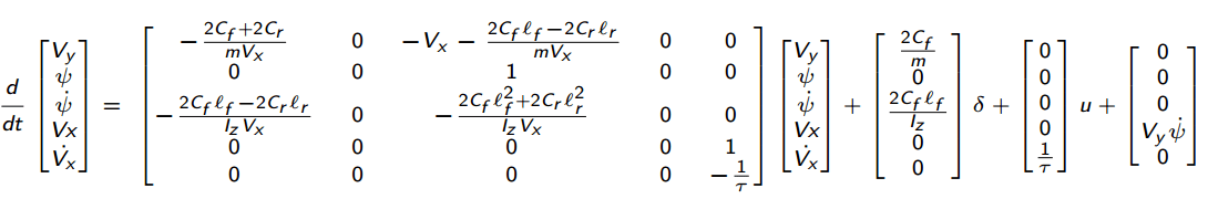
In the state vector,  denotes the lateral velocity, denotes the longitudinal velocity and
  denotes the yaw angle. The vehicle parameters are provided in the
 helperACCSetUp file.
The outputs from the vehicle dynamics (such as longitudinal velocity and lateral velocity ) are based on body fixed coordinates. To obtain the trajectory traversed by the vehicle, the body fixed coordinates are converted into global coordinates through the following relations:

The yaw angle and yaw angle rate  are also converted into the units of degrees.
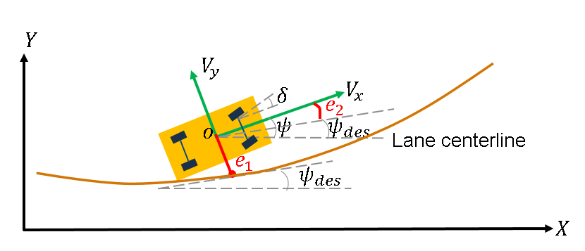
The goal for the driver steering model is to keep the vehicle in its lane and follow the curved road by controlling the front steering angle . This goal is achieved by driving the yaw angle error  and lateral displacement error
  to zero (see the following figure), where

The desired yaw angle rate is given by  (
( denotes the radius for the road curvature).
The Actors and Sensor Simulation subsystem generates the synthetic sensor data required for tracking and sensor fusion. Before running this example, the Driving Scenario Designer app was used to create a scenario with a curved road and multiple actors moving on the road. The roads and actors from this scenario were then exported to the MATLAB function ACCTestBenchScenario.m. To see how you can define the scenario, see the Scenario Creation section.
open_system('ACCTestBenchExample/Vehicle and Environment/Actors and Sensor Simulation')
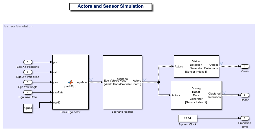
The motion of the ego vehicle is controlled by the control system and is not read from the scenario file. Instead, the ego vehicle position, velocity, yaw angle, and yaw rate are received as inputs from the Vehicle Dynamics block and are packed into a single actor pose structure using the packEgo MATLAB function block.
The Scenario Reader block reads the actor pose data from the scenario variable loaded in the workspace. The model runs ACCTestBenchScenario.m to load the scenario into the workspace at the start of simulation. You can also load the scenario by clicking the Run Scenario Script button in the model. The block converts the actor poses from the world coordinates of the scenario into ego vehicle coordinates. The actor poses are streamed on a bus generated by the block. In this example, you use a Vision Detection Generator block and Radar Detection Generator block. Both sensors are long-range and forward-looking, and provide good coverage of the front of the ego vehicle, as needed for ACC. The sensors use the actor poses in ego vehicle coordinates to generate lists of vehicle detections in front of the ego vehicle. Finally, a clock block is used as an example of how the vehicle would have a centralized time source. The time is used by the Multi-Object Tracker block.
Scenario Creation
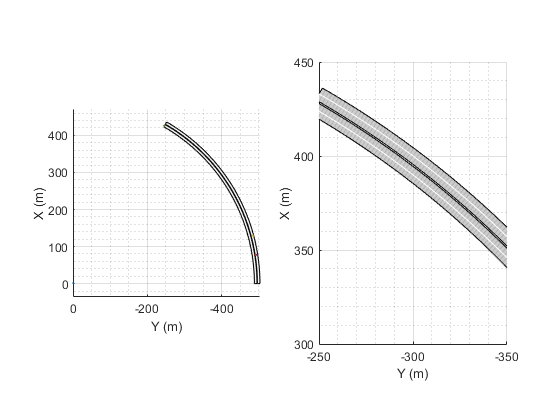
The Driving Scenario Designer app allows you to define roads and vehicles moving on the roads. For this example, you define two parallel roads of constant curvature. To define the road, you define the road centers, the road width, and banking angle (if needed). The road centers were chosen by sampling points along a circular arc, spanning a turn of 60 degrees of constant radius of curvature.
You define all the vehicles in the scenario. To define the motion of the vehicles, you define their trajectory by a set of waypoints and speeds. A quick way to define the waypoints is by choosing a subset of the road centers defined earlier, with an offset to the left or right of the road centers to control the lane in which the vehicles travel.
This example shows four vehicles: a fast-moving car in the left lane, a slow-moving car in the right lane, a car approaching on the opposite side of the road, and a car that starts on the right lane, but then moves to the left lane to pass the slow-moving car.
The scenario can be modified using the Driving Scenario Designer app and exported and saved to the same scenario file ACCTestBenchScenario.m. The Scenario Reader block automatically picks up the changes when simulation is rerun. To build the scenario programmatically, you can use the helperScenarioAuthoring function.
plotACCScenario
Generating Code for the Control Algorithm
Although the entire model does not support code generation, the ACCWithSensorFusionMdlRef model is configured to support generating C code using Embedded Coder software. To check if you have access to Embedded Coder, run:
hasEmbeddedCoderLicense = license('checkout','RTW_Embedded_Coder')
You can generate a C function for the model and explore the code generation report by running:
if hasEmbeddedCoderLicense
    slbuild('ACCWithSensorFusionMdlRef')
end
You can verify that the compiled C code behaves as expected using software-in-the-loop (SIL) simulation. To simulate the ACCWithSensorFusionMdlRef referenced model in SIL mode, use:
if hasEmbeddedCoderLicense
    set_param('ACCTestBenchExample/ACC with Sensor Fusion',...
        'SimulationMode','Software-in-the-loop (SIL)')
end
When you run the ACCTestBenchExample model, code is generated, compiled, and executed for the ACCWithSensorFusionMdlRef model. This enables you to test the behavior of the compiled code through simulation.
Conclusions
This example shows how to implement an integrated adaptive cruise controller (ACC) on a curved road with sensor fusion, test it in Simulink using synthetic data generated by the Automated Driving Toolbox, componentize it, and automatically generate code for it.
% Close any systems opened during execution of this example.
endingOpenSystems = find_system('MatchFilter', @Simulink.match.allVariants);
bdclose(setdiff(endingOpenSystems,startingOpenSystems))
See Also
Functions
Blocks
- Vision Detection Generator | Driving Radar Data Generator | Detection Concatenation | Multi-Object Tracker | Adaptive Cruise Control System (Model Predictive Control Toolbox)