Adaptive MPC Control of Nonlinear Chemical Reactor Using Successive Linearization
This example shows how to use an Adaptive MPC controller to control a nonlinear continuous stirred tank reactor (CSTR) as it transitions from low conversion rate to high conversion rate.
A first principle nonlinear plant model is available and being linearized at each control interval. The adaptive MPC controller then updates its internal predictive model with the linearized plant model and achieves nonlinear control successfully.
About the Continuous Stirred Tank Reactor
A Continuously Stirred Tank Reactor (CSTR) is a common chemical system in the process industry. A schematic of the CSTR system is:

This is a jacketed non-adiabatic tank reactor described extensively in Seborg's book, "Process Dynamics and Control", published by Wiley, 2004. The vessel is assumed to be perfectly mixed, and a single first-order exothermic and irreversible reaction, A --> B, takes place. The inlet stream of reagent A is fed to the tank at a constant volumetric rate. The product stream exits continuously at the same volumetric rate and liquid density is constant. Thus the volume of reacting liquid is constant.
The inputs of the CSTR model are:
![$$ \begin{array} {ll} u_1 = CA_i \; & \textnormal{Concentration of A in inlet feed stream} [kmol/m^3] \\ u_2 = T_i \; & \textnormal{Inlet feed stream temperature} [K] \\ u_3 = T_c \; & \textnormal{Jacket coolant temperature} [K] \\ \end{array} $$](../../examples/mpc/win64/ampccstr_linearization_eq15339119666843927976.png)
and the outputs (y(t)), which are also the states of the model (x(t)), are:
![$$ \begin{array} {ll} y_1 = x_1 = CA \; & \textnormal{Concentration of A in reactor tank} [kmol/m^3] \\ y_2 = x_2 = T \; & \textnormal{Reactor temperature} [K] \\ \end{array} $$](../../examples/mpc/win64/ampccstr_linearization_eq16596258212567713182.png)
The control objective is to maintain the concentration of reagent A,  at its desired setpoint, which changes over time when reactor transitions from low conversion rate to high conversion rate. The coolant temperature
  is the manipulated variable used by the MPC controller to track the reference as well as reject the measured disturbance arising from the inlet feed stream temperature
  . The inlet feed stream concentration,
  , is assumed to be constant. The Simulink® model
 mpc_cstr_plant implements the nonlinear CSTR plant.
We also assume that direct measurements of concentrations are unavailable or infrequent, which is the usual case in practice. Instead, we use a "soft sensor" to estimate CA based on temperature measurements and the plant model. For more information on the CSTR reactor and related examples, see CSTR Model.
About Adaptive Model Predictive Control
It is well known that the CSTR dynamics are strongly nonlinear with respect to reactor temperature variations and can be open-loop unstable during the transition from one operating condition to another. A single MPC controller designed at a particular operating condition cannot give satisfactory control performance over a wide operating range.
To control the nonlinear CSTR plant with linear MPC control technique, you have a few options:
If a linear plant model cannot be obtained at run time, first you need to obtain several linear plant models offline at different operating conditions that cover the typical operating range. Next you can choose one of the two approaches to implement MPC control strategy:
(1) Design several MPC controllers offline, one for each plant model. At run time, use Multiple MPC Controller block that switches MPC controllers from one to another based on a desired scheduling strategy. For more details, see Gain-Scheduled MPC Control of Nonlinear Chemical Reactor. Use this approach when the plant models have different orders or time delays.
(2) Design one MPC controller offline at the initial operating point. At run time, use Adaptive MPC Controller block (updating predictive model at each control interval) together with Linear Parameter Varying (LPV) System block (supplying linear plant model with a scheduling strategy). See Adaptive MPC Control of Nonlinear Chemical Reactor Using Linear Parameter-Varying System for more details. Use this approach when all the plant models have the same order and time delay.
If a linear plant model can be obtained at run time, you should use Adaptive MPC Controller block to achieve nonlinear control. There are two typical ways to obtain a linear plant model online:
(1) Use successive linearization as shown in this example. Use this approach when a nonlinear plant model is available and can be linearized at run time.
(2) Use online estimation to identify a linear model when loop is closed. See Adaptive MPC Control of Nonlinear Chemical Reactor Using Online Model Estimation for more details. Use this approach when linear plant model cannot be obtained from either an LPV system or successive linearization.
Obtain Linear Plant Model at Initial Operating Condition
To implement an adaptive MPC controller, first you need to design an MPC controller at the initial operating point where CAi is 10 kmol/m^3, Ti and Tc are 298.15 K.
Create operating point specification.
plant_mdl = 'mpc_cstr_plant';
op = operspec(plant_mdl);
Feed concentration is known at the initial condition.
op.Inputs(1).u = 10;
op.Inputs(1).Known = true;
Feed temperature is known at the initial condition.
op.Inputs(2).u = 298.15;
op.Inputs(2).Known = true;
Coolant temperature is known at the initial condition.
op.Inputs(3).u = 298.15;
op.Inputs(3).Known = true;
Compute initial condition.
[op_point, op_report] = findop(plant_mdl,op);
 Operating point search report:
---------------------------------

opreport =


 Operating point search report for the Model mpc_cstr_plant.
 (Time-Varying Components Evaluated at time t=0)

Operating point specifications were successfully met.
States:
----------
    Min          x          Max        dxMin        dx         dxMax
___________ ___________ ___________ ___________ ___________ ___________

(1.) mpc_cstr_plant/CSTR/Integrator
     0       311.2639       Inf          0      8.1176e-11       0
(2.) mpc_cstr_plant/CSTR/Integrator1
     0        8.5698        Inf          0      -6.8709e-12      0

Inputs:
----------
 Min     u     Max
______ ______ ______

(1.) mpc_cstr_plant/CAi
  10     10     10
(2.) mpc_cstr_plant/Ti
298.15 298.15 298.15
(3.) mpc_cstr_plant/Tc
298.15 298.15 298.15

Outputs:
----------
  Min       y       Max
________ ________ ________

(1.) mpc_cstr_plant/T
  -Inf   311.2639   Inf
(2.) mpc_cstr_plant/CA
  -Inf    8.5698    Inf
Obtain nominal values of x, y and u.
x0 = [op_report.States(1).x;op_report.States(2).x];
y0 = [op_report.Outputs(1).y;op_report.Outputs(2).y];
u0 = [op_report.Inputs(1).u;op_report.Inputs(2).u;op_report.Inputs(3).u];
Obtain linear plant model at the initial condition.
sys = linearize(plant_mdl, op_point);
Drop the first plant input CAi because it is not used by MPC.
sys = sys(:,2:3);
Discretize the plant model because Adaptive MPC controller only accepts a discrete-time plant model.
Ts = 0.5;
plant = c2d(sys,Ts);
Design MPC Controller
You design an MPC at the initial operating condition. When running in the adaptive mode, the plant model is updated at run time.
Specify signal types used in MPC.
plant.InputGroup.MeasuredDisturbances = 1;
plant.InputGroup.ManipulatedVariables = 2;
plant.OutputGroup.Measured = 1;
plant.OutputGroup.Unmeasured = 2;
plant.InputName = {'Ti','Tc'};
plant.OutputName = {'T','CA'};
Create MPC controller with default prediction and control horizons.
mpcobj = mpc(plant);
-->"PredictionHorizon" is empty. Assuming default 10.
-->"ControlHorizon" is empty. Assuming default 2.
-->"Weights.ManipulatedVariables" is empty. Assuming default 0.00000.
-->"Weights.ManipulatedVariablesRate" is empty. Assuming default 0.10000.
-->"Weights.OutputVariables" is empty. Assuming default 1.00000.
   for output(s) y1 and zero weight for output(s) y2
Set nominal values in the controller.
mpcobj.Model.Nominal = struct('X', x0, 'U', u0(2:3), 'Y', y0, 'DX', [0 0]);
Set scale factors because plant input and output signals have different orders of magnitude.
Uscale = [30 50];
Yscale = [50 10];
mpcobj.DV(1).ScaleFactor = Uscale(1);
mpcobj.MV(1).ScaleFactor = Uscale(2);
mpcobj.OV(1).ScaleFactor = Yscale(1);
mpcobj.OV(2).ScaleFactor = Yscale(2);
Let reactor temperature T float (i.e. with no setpoint tracking error penalty), because the objective is to control reactor concentration CA and only one manipulated variable (coolant temperature Tc) is available.
mpcobj.Weights.OV = [0 1];
Due to the physical constraint of coolant jacket, Tc rate of change is bounded by degrees per minute.
mpcobj.MV.RateMin = -2;
mpcobj.MV.RateMax = 2;
Implement Adaptive MPC Control of CSTR Plant in Simulink
Open the Simulink model.
mdl = 'ampc_cstr_linearization';
open_system(mdl)
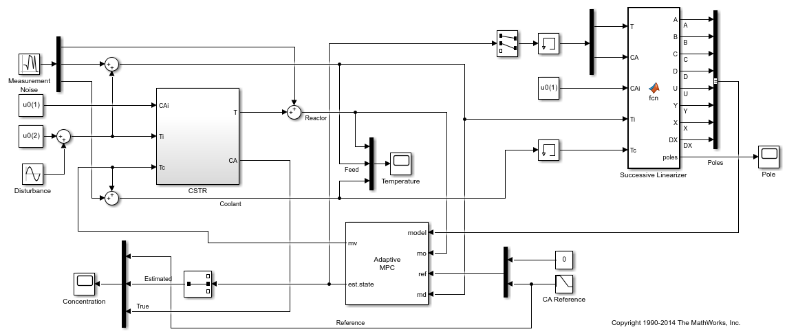
The model includes three parts:
The "CSTR" block implements the nonlinear plant model.
The "Adaptive MPC Controller" block runs the designed MPC controller in the adaptive mode.
The "Successive Linearizer" block in a MATLAB Function block that linearizes a first principle nonlinear CSTR plant and provides the linear plant model to the "Adaptive MPC Controller" block at each control interval. Double click the block to see the MATLAB® code. You can use the block as a template to develop appropriate linearizer for your own applications.
Note that the new linear plant model must be a discrete time state space system with the same order and sample time as the original plant model has. If the plant has time delay, it must also be same as the original time delay and absorbed into the state space model.
Validate Adaptive MPC Control Performance
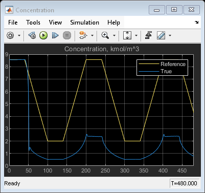
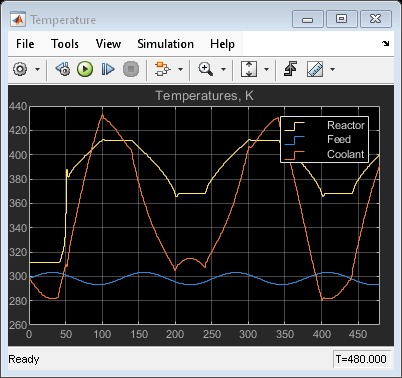
Controller performance is validated against both setpoint tracking and disturbance rejection.
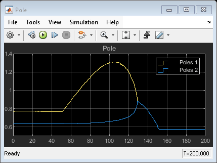
Tracking: reactor concentration CA setpoint transitions from original 8.57 (low conversion rate) to 2 (high conversion rate) kmol/m^3. During the transition, the plant first becomes unstable then stable again (see the poles plot).
Regulating: feed temperature Ti has slow fluctuation represented by a sine wave with amplitude of 5 degrees, which is a measured disturbance fed to the MPC controller.
Simulate the closed-loop performance.
open_system([mdl '/Concentration'])
open_system([mdl '/Temperature'])
open_system([mdl '/Pole'])
sim(mdl)
-->Assuming output disturbance added to measured output #1 is integrated white noise.
-->"Model.Noise" is empty. Assuming white noise on each measured output.
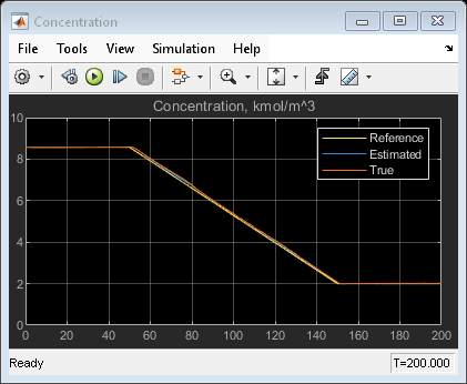

The tracking and regulating performance is very satisfactory. In an application to a real reactor, however, model inaccuracies and unmeasured disturbances could cause poorer tracking than shown here. Additional simulations could be used to study these effects.
Compare with Non-Adaptive MPC Control
Adaptive MPC provides superior control performance than a non-adaptive MPC. To illustrate this point, the control performance of the same MPC controller running in the non-adaptive mode is shown below. The controller is implemented with an MPC Controller block.
mdl1 = 'ampc_cstr_no_linearization';
open_system(mdl1)
open_system([mdl1 '/Concentration'])
open_system([mdl1 '/Temperature'])
sim(mdl1)
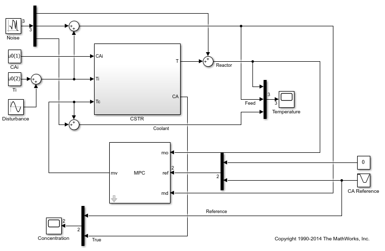
As expected, the tracking and regulating performance of non-adaptive MPC is not acceptable.
See Also
Functions
Objects
mpc|mpcstate|mpcmoveopt